Jaws: Repeated Measures Analysis of Variance
An example from OpenBUGS [44] and Elston and Grizzle [24] concerning jaw bone heights measured repeatedly in a cohort of 20 boys at ages 8, 8.5, 9, and 9.5 years.
Model
Bone heights are modelled as
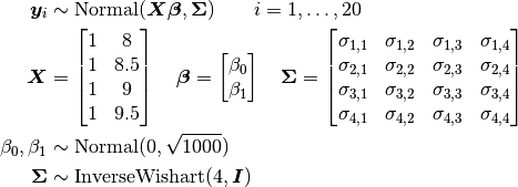
where  is a vector of the four repeated measurements for boy
  . In the model specification below, bone heights are arranged into a 1-dimensional vector on which a Block-Diagonal Multivariate Normal Distribution is specified. Also not that since
  is a covariance matrix, it is symmetric with
 M * (M + 1) / 2 unique (upper or lower triangular) parameters, where M is the matrix dimension.
Analysis Program
using Distributed
@everywhere using Mamba, LinearAlgebra

## Data
jaws = Dict{Symbol, Any}(
  :Y =>
   [47.8 48.8 49.0 49.7
    46.4 47.3 47.7 48.4
    46.3 46.8 47.8 48.5
    45.1 45.3 46.1 47.2
    47.6 48.5 48.9 49.3
    52.5 53.2 53.3 53.7
    51.2 53.0 54.3 54.5
    49.8 50.0 50.3 52.7
    48.1 50.8 52.3 54.4
    45.0 47.0 47.3 48.3
    51.2 51.4 51.6 51.9
    48.5 49.2 53.0 55.5
    52.1 52.8 53.7 55.0
    48.2 48.9 49.3 49.8
    49.6 50.4 51.2 51.8
    50.7 51.7 52.7 53.3
    47.2 47.7 48.4 49.5
    53.3 54.6 55.1 55.3
    46.2 47.5 48.1 48.4
    46.3 47.6 51.3 51.8],
  :age => [8.0, 8.5, 9.0, 9.5]
)
M = jaws[:M] = size(jaws[:Y], 2)
N = jaws[:N] = size(jaws[:Y], 1)
jaws[:y] = vec(jaws[:Y])
jaws[:x] = kron(ones(jaws[:N]), jaws[:age])


## Model Specification
model = Model(

  y = Stochastic(1,
    (beta0, beta1, x, Sigma) -> BDiagNormal(beta0 .+ beta1 * x, Sigma),
    false
  ),

  beta0 = Stochastic(
    () -> Normal(0, sqrt(1000))
  ),

  beta1 = Stochastic(
    () -> Normal(0, sqrt(1000))
  ),

  Sigma = Stochastic(2,
    M -> InverseWishart(4.0, Matrix{Float64}(I, M, M))
  )

)


## Initial Values
inits = [
  Dict(:y => jaws[:y], :beta0 => 40, :beta1 => 1, :Sigma => Matrix{Float64}(I, M, M)),
  Dict(:y => jaws[:y], :beta0 => 10, :beta1 => 10, :Sigma => Matrix{Float64}(I, M, M))
]


## Sampling Scheme
scheme = [Slice([:beta0, :beta1], [10, 1]),
          AMWG(:Sigma, 0.1)]
setsamplers!(model, scheme)


## MCMC Simulations
sim = mcmc(model, jaws, inits, 10000, burnin=2500, thin=2, chains=2)
describe(sim)
Results
Iterations = 2502:10000
Thinning interval = 2
Chains = 1,2
Samples per chain = 3750

Empirical Posterior Estimates:
              Mean        SD      Naive SE       MCSE        ESS
Sigma[1,1]  6.7915801 2.0232463 0.0233624358 0.1421847433 202.48437
Sigma[1,2]  6.5982624 1.9670001 0.0227129612 0.1469366529 179.20433
Sigma[1,3]  6.1775526 1.9084389 0.0220367541 0.1532226770 155.13523
Sigma[1,4]  5.9477070 1.9358258 0.0223529913 0.1545185214 156.95367
Sigma[2,2]  6.9308723 2.0236387 0.0233669666 0.1531630007 174.56542
Sigma[2,3]  6.6005767 1.9885583 0.0229618936 0.1600864592 154.30055
Sigma[2,4]  6.3803028 2.0196017 0.0233203515 0.1612393116 156.88795
Sigma[3,3]  7.4564163 2.1925641 0.0253175499 0.1705734202 165.22733
Sigma[3,4]  7.4518620 2.2712194 0.0262257824 0.1733769737 171.60713
Sigma[4,4]  8.0594440 2.4746352 0.0285746264 0.1784057891 192.39975
     beta1  1.8742617 0.2272166 0.0026236712 0.0071954415 997.16079
     beta0 33.6379701 1.9912509 0.0229929845 0.0632742554 990.37090

Quantiles:
              2.5%       25.0%      50.0%      75.0%      97.5%
Sigma[1,1]  3.7202164  5.3419070  6.5046777  7.8684049 11.5279247
Sigma[1,2]  3.5674344  5.2009878  6.3564397  7.6419462 11.2720602
Sigma[1,3]  3.2043099  4.8527075  5.9476859  7.1929746 10.8427648
Sigma[1,4]  2.9143241  4.5808041  5.6958961  6.9962164 10.6253935
Sigma[2,2]  3.7936234  5.4940524  6.6730872  8.0151463 11.6796110
Sigma[2,3]  3.4721419  5.2183567  6.3620683  7.6617912 11.4419940
Sigma[2,4]  3.2133129  4.9659531  6.1310937  7.4443619 11.3714037
Sigma[3,3]  4.1213458  5.9139585  7.1780478  8.6551856 12.8617596
Sigma[3,4]  4.0756709  5.8561719  7.1240011  8.7006336 13.0597624
Sigma[4,4]  4.4482953  6.3090779  7.6484712  9.4043857 14.0451233
     beta1  1.4349627  1.7279142  1.8707215  2.0159440  2.3445976
     beta0 29.4960557 32.3922780 33.6327451 34.9577696 37.4067853