Dogs: Loglinear Model for Binary Data
An example from OpenBUGS [44], Lindley and Smith [54], and Kalbfleisch [52] concerning the Solomon-Wynne experiment on dogs. In the experiment, 30 dogs were subjected to 25 trials. On each trial, a barrier was raised, and an electric shock was administered 10 seconds later if the dog did not jump the barrier.
Model
Failures to jump the barriers in time are modelled as
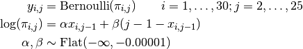
where  if dog
  fails to jump the barrier before the shock on trial
  , and 0 otherwise;
  is the number of successful jumps prior to trial ; and
  is the probability of failure.
Analysis Program
using Mamba

## Data
dogs = Dict{Symbol, Any}(
  :Y =>
    [0 0 1 0 1 0 1 1 1 1 1 1 1 1 1 1 1 1 1 1 1 1 1 1 1
     0 0 0 0 0 0 0 1 0 0 0 0 0 0 0 1 1 1 1 1 1 1 1 1 1
     0 0 0 0 0 1 1 0 1 1 0 0 1 1 0 1 0 1 1 1 1 1 1 1 1
     0 1 1 0 0 1 1 1 1 0 1 0 1 0 1 1 1 1 1 1 1 1 1 1 1
     0 0 0 0 0 0 0 0 1 1 1 1 1 1 1 1 1 1 1 1 1 1 1 1 1
     0 0 0 0 0 0 1 1 1 1 0 0 1 0 1 1 1 1 1 1 1 1 1 1 1
     0 0 0 0 0 1 0 0 0 0 0 0 1 1 1 1 1 1 1 1 1 1 1 1 1
     0 0 0 0 0 0 0 1 1 0 0 1 1 1 1 1 1 1 1 1 1 1 1 1 1
     0 0 0 0 0 1 0 1 0 1 1 0 1 0 0 0 1 1 1 1 1 0 1 1 0
     0 0 0 0 1 0 0 1 1 0 1 0 1 1 1 1 1 1 1 1 1 1 1 1 1
     0 0 0 0 0 0 0 0 0 0 1 1 1 1 1 1 1 1 1 1 1 1 1 1 1
     0 0 0 0 0 1 1 1 1 1 0 0 1 1 1 1 1 1 1 1 1 1 1 1 1
     0 0 0 1 1 0 1 0 0 1 1 1 1 1 1 1 1 1 1 1 1 1 1 1 1
     0 0 0 0 1 0 1 1 0 1 1 1 1 1 1 1 1 1 1 1 1 1 1 1 1
     0 0 0 1 0 1 1 0 1 1 1 1 1 1 1 1 1 1 1 1 1 1 1 1 1
     0 0 0 0 0 0 0 1 1 1 1 1 1 1 1 1 1 1 1 1 1 1 1 1 1
     0 1 0 1 0 0 0 1 0 1 1 1 1 0 1 1 1 1 1 1 1 1 1 1 1
     0 0 0 0 1 0 1 0 1 1 1 1 1 0 1 1 1 1 1 1 1 1 1 1 1
     0 1 0 0 0 0 1 0 0 0 1 1 1 1 1 1 1 1 1 1 1 1 1 1 1
     0 0 0 0 1 1 0 1 0 1 1 0 1 0 1 1 1 1 1 1 1 1 1 1 1
     0 0 0 1 1 1 1 1 0 1 1 1 1 1 1 1 1 1 1 1 1 1 1 1 1
     0 0 1 0 1 0 1 1 1 1 1 1 1 1 1 1 0 0 1 1 1 1 1 1 1
     0 0 0 0 0 0 0 1 1 1 1 1 1 1 1 1 1 1 1 1 1 1 1 1 1
     0 0 0 0 0 0 0 0 1 1 1 0 1 0 0 0 1 1 0 1 1 1 1 1 1
     0 0 0 0 0 0 1 1 0 1 1 1 0 1 0 1 1 1 1 1 1 1 1 1 1
     0 0 1 0 1 1 1 0 1 1 0 1 1 1 1 1 1 1 1 1 1 1 1 1 1
     0 0 0 0 1 0 1 1 1 1 1 1 1 1 1 1 1 1 1 1 1 1 1 1 1
     0 0 0 1 0 1 0 1 1 1 0 1 1 1 1 1 1 1 1 1 1 1 1 1 1
     0 0 0 0 1 1 0 0 1 1 1 0 1 0 1 0 1 0 1 1 1 1 1 1 1
     0 0 0 0 1 1 1 1 1 1 0 1 0 1 1 1 1 1 1 1 1 1 1 1 1]
)
dogs[:Dogs] = size(dogs[:Y], 1)
dogs[:Trials] = size(dogs[:Y], 2)

dogs[:xa] = mapslices(cumsum, dogs[:Y], 2)
dogs[:xs] = mapslices(x -> collect(1:25) - x, dogs[:xa], 2)
dogs[:y] = 1 - dogs[:Y][:, 2:25]


## Model Specification
model = Model(

  y = Stochastic(2,
    (Dogs, Trials, alpha, xa, beta, xs) ->
      UnivariateDistribution[
        begin
          p = exp(alpha * xa[i, j] + beta * xs[i, j])
          Bernoulli(p)
        end
        for i in 1:Dogs, j in 1:Trials-1
      ],
    false
  ),

  alpha = Stochastic(
    () -> Truncated(Flat(), -Inf, -1e-5)
  ),

  A = Logical(
    alpha -> exp(alpha)
  ),

  beta = Stochastic(
    () -> Truncated(Flat(), -Inf, -1e-5)
  ),

  B = Logical(
    beta -> exp(beta)
  )

)


## Initial Values
inits = [
  Dict(:y => dogs[:y], :alpha => -1, :beta => -1),
  Dict(:y => dogs[:y], :alpha => -2, :beta => -2)
]


## Sampling Scheme
scheme = [Slice([:alpha, :beta], 1.0)]
setsamplers!(model, scheme)


## MCMC Simulations
sim = mcmc(model, dogs, inits, 10000, burnin=2500, thin=2, chains=2)
describe(sim)
Results
Iterations = 2502:10000
Thinning interval = 2
Chains = 1,2
Samples per chain = 3750

Empirical Posterior Estimates:
         Mean         SD        Naive SE        MCSE        ESS
 beta -0.0788601 0.011812880 0.00013640339 0.00018435162 3750.0000
    B  0.9242336 0.010903201 0.00012589932 0.00017012187 3750.0000
alpha -0.2441654 0.024064384 0.00027787158 0.00045249868 2828.2310
    A  0.7835846 0.018821132 0.00021732772 0.00035466850 2816.0882

Quantiles:
          2.5%        25.0%       50.0%       75.0%       97.5%
 beta -0.10326776 -0.086633844 -0.07848501 -0.07046663 -0.05703080
    B  0.90188545  0.917012804  0.92451592  0.93195884  0.94456498
alpha -0.29269315 -0.260167645 -0.24381478 -0.22784322 -0.19872975
    A  0.74625110  0.770922334  0.78363276  0.79624909  0.81977141