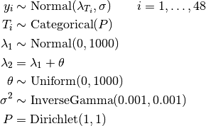
Eyes: Normal Mixture Model
An example from OpenBUGS [44], Bowmaker [7], and Robert [77] concerning 48 peak sensitivity wavelength measurements taken on a set of monkey’s eyes.
 is the measurement on monkey
  .
.Analysis Program
using Distributed
@everywhere using Mamba

## Data
eyes = Dict{Symbol, Any}(
  :y =>
    [529.0, 530.0, 532.0, 533.1, 533.4, 533.6, 533.7, 534.1, 534.8, 535.3,
     535.4, 535.9, 536.1, 536.3, 536.4, 536.6, 537.0, 537.4, 537.5, 538.3,
     538.5, 538.6, 539.4, 539.6, 540.4, 540.8, 542.0, 542.8, 543.0, 543.5,
     543.8, 543.9, 545.3, 546.2, 548.8, 548.7, 548.9, 549.0, 549.4, 549.9,
     550.6, 551.2, 551.4, 551.5, 551.6, 552.8, 552.9, 553.2],
  :N => 48,
  :alpha => [1, 1]
)


## Model Specification
model = Model(

  y = Stochastic(1,
    (lambda, T, s2, N) ->
      begin
        sigma = sqrt(s2)
        UnivariateDistribution[(
          mu = lambda[Int(T[i])];
          Normal(mu, sigma)) for i in 1:N
        ]
      end,
    false
  ),

  T = Stochastic(1,
    (P, N) -> UnivariateDistribution[Categorical(P) for i in 1:N],
    false
  ),

  P = Stochastic(1,
    alpha -> Dirichlet(alpha)
  ),

  lambda = Logical(1,
    (lambda0, theta) -> Float64[lambda0; lambda0 + theta]
  ),

  lambda0 = Stochastic(
    () -> Normal(0.0, 1000.0),
    false
  ),

  theta = Stochastic(
    () -> Uniform(0.0, 1000.0),
    false
  ),

  s2 = Stochastic(
    () -> InverseGamma(0.001, 0.001)
  )

)


## Initial Values
inits = [
  Dict(:y => eyes[:y], :T => fill(1, eyes[:N]), :P => [0.5, 0.5],
       :lambda0 => 535, :theta => 5, :s2 => 10),
  Dict(:y => eyes[:y], :T => fill(1, eyes[:N]), :P => [0.5, 0.5],
       :lambda0 => 550, :theta => 1, :s2 => 1)
]


## Sampling Scheme
scheme = [DGS(:T),
          Slice([:lambda0, :theta], [5.0, 1.0]),
          Slice(:s2, 2.0, transform=true),
          SliceSimplex(:P, scale=0.75)]
setsamplers!(model, scheme)


## MCMC Simulations
sim = mcmc(model, eyes, inits, 10000, burnin=2500, thin=2, chains=2)
describe(sim)
Results
Iterations = 2502:10000
Thinning interval = 2
Chains = 1,2
Samples per chain = 3750

Empirical Posterior Estimates:
              Mean         SD       Naive SE       MCSE         ESS
     P[1]   0.60357102 0.08379221 0.0009675491 0.0013077559 3750.00000
     P[2]   0.39642898 0.08379221 0.0009675491 0.0013077559 3750.00000
       s2  14.45234459 4.96689604 0.0573527753 0.1853970211  717.73584
lambda[1] 536.75250337 0.88484533 0.0102173137 0.0304232594  845.90821
lambda[2] 548.98693469 1.18938418 0.0137338256 0.0625489045  361.58042

Quantiles:
              2.5%         25.0%        50.0%        75.0%        97.5%
     P[1]   0.43576584   0.54842468   0.60395494   0.66066383   0.76552882
     P[2]   0.23447118   0.33933617   0.39604506   0.45157532   0.56423416
       s2   8.55745263  11.37700782  13.39622105  16.26405571  27.08863166
lambda[1] 535.08951002 536.16891895 536.73114152 537.30710397 538.61179506
lambda[2] 546.57859195 548.24188698 548.97732892 549.74377421 551.38780148