Dyes: Variance Components Model¶

An example from OpenBUGS [38], Davies [18], and Box and Tiao [7] concerning batch-to-batch variation in yields from six batches and five samples of dyestuff.

Model¶

Yields are modelled as

$y_{i,j} &\sim \text{Normal}(\mu_i, \sigma_\text{within}) \quad\quad i=1,\ldots,6; j=1,\ldots,5 \\ \mu_i &\sim \text{Normal}(\theta, \sigma_\text{between}) \\ \theta &\sim \text{Normal}(0, 1000) \\ \sigma^2_\text{within}, \sigma^2_\text{between} &\sim \text{InverseGamma}(0.001, 0.001),$

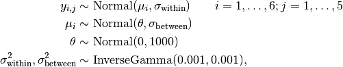
where $y_{i,j}$ is the response for batch $i$ and sample $j$ .

Analysis Program¶

using Mamba

## Data
dyes = (Symbol => Any)[
  :y =>
    [1545, 1440, 1440, 1520, 1580,
     1540, 1555, 1490, 1560, 1495,
     1595, 1550, 1605, 1510, 1560,
     1445, 1440, 1595, 1465, 1545,
     1595, 1630, 1515, 1635, 1625,
     1520, 1455, 1450, 1480, 1445],
  :batches => 6,
  :samples => 5
]

dyes[:batch] = vcat([fill(i, dyes[:samples]) for i in 1:dyes[:batches]]...)
dyes[:sample] = vcat(fill([1:dyes[:samples]], dyes[:batches])...)


## Model Specification

model = Model(

  y = Stochastic(1,
    @modelexpr(mu, batch, s2_within,
      MvNormal(mu[batch], sqrt(s2_within))
    ),
    false
  ),

  mu = Stochastic(1,
    @modelexpr(theta, batches, s2_between,
      Normal(theta, sqrt(s2_between))
    ),
    false
  ),

  theta = Stochastic(
    :(Normal(0, 1000))
  ),

  s2_within = Stochastic(
    :(InverseGamma(0.001, 0.001))
  ),

  s2_between = Stochastic(
    :(InverseGamma(0.001, 0.001))
  )

)


## Initial Values
inits = [
  [:y => dyes[:y], :theta => 1500, :s2_within => 1, :s2_between => 1,
   :mu => fill(1500, dyes[:batches])],
  [:y => dyes[:y], :theta => 3000, :s2_within => 10, :s2_between => 10,
   :mu => fill(3000, dyes[:batches])]
]


## Sampling Scheme
scheme = [NUTS([:mu, :theta]),
          Slice([:s2_within, :s2_between], [1000.0, 1000.0])]
setsamplers!(model, scheme)


## MCMC Simulations
sim = mcmc(model, dyes, inits, 10000, burnin=2500, thin=2, chains=2)
describe(sim)

Results¶

Iterations = 2502:10000
Thinning interval = 2
Chains = 1,2
Samples per chain = 3750

Empirical Posterior Estimates:
              Mean       SD     Naive SE    MCSE       ESS
s2_between 2504.9567 2821.1909 32.576307 201.76845  195.50525
 s2_within 2870.5356  997.8584 11.522276  50.36398  392.55247
     theta 1527.0634   22.9340  0.264819   0.39541 3363.98979

Quantiles:
               2.5%      25.0%     50.0%    75.0%       97.5%
s2_between  152.111234  850.5886 1676.491 3000.7898 1.287454x104
 s2_within 1532.847859 2175.9060 2665.165 3328.3947  5.54381x103
     theta 1481.227885 1512.8876 1527.653 1540.3759  1.57204x103