Jaws: Repeated Measures Analysis of Variance¶

An example from OpenBUGS [38] and Elston and Grizzle [20] concerning jaw bone heights measured repeatedly in a cohort of 20 boys at ages 8, 8.5, 9, and 9.5 years.

Model¶

Bone heights are modelled as

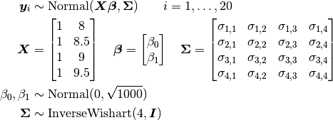
$\bm{y}_i &\sim \text{Normal}(\bm{X} \bm{\beta}, \bm{\Sigma}) \quad\quad i=1,\ldots,20 \\ \bm{X} &= \begin{bmatrix} 1 & 8 \\ 1 & 8.5 \\ 1 & 9 \\ 1 & 9.5 \\ \end{bmatrix} \quad \bm{\beta} = \begin{bmatrix} \beta_0 \\ \beta_1 \\ \end{bmatrix} \quad \bm{\Sigma} = \begin{bmatrix} \sigma_{1,1} & \sigma_{1,2} & \sigma_{1,3} & \sigma_{1,4} \\ \sigma_{2,1} & \sigma_{2,2} & \sigma_{2,3} & \sigma_{2,4} \\ \sigma_{3,1} & \sigma_{3,2} & \sigma_{3,3} & \sigma_{3,4} \\ \sigma_{4,1} & \sigma_{4,2} & \sigma_{4,3} & \sigma_{4,4} \\ \end{bmatrix} \\ \beta_0, \beta_1 &\sim \text{Normal}(0, \sqrt{1000}) \\ \bm{\Sigma} &\sim \text{InverseWishart}(4, \bm{I})$

where $\bm{y}_i$ is a vector of the four repeated measurements for boy $i$ . In the model specification below, the bone heights are arranged into a 1-dimensional vector on which a Block-Diagonal Multivariate Normal Distribution is specified. Furthermore, since $\bm{\Sigma}$ is a covariance matrix, it is symmetric with M * (M + 1) / 2 unique (upper or lower triangular) parameters, where M is the matrix dimension. Consequently, that is the number of parameters to account for when defining samplers for $\bm{\Sigma}$ ; e.g., AMWG([:Sigma], fill(0.1, int(M * (M + 1) / 2))).

Analysis Program¶

using Mamba

## Data
jaws = (Symbol => Any)[
  :Y =>
   [47.8 48.8 49.0 49.7
    46.4 47.3 47.7 48.4
    46.3 46.8 47.8 48.5
    45.1 45.3 46.1 47.2
    47.6 48.5 48.9 49.3
    52.5 53.2 53.3 53.7
    51.2 53.0 54.3 54.5
    49.8 50.0 50.3 52.7
    48.1 50.8 52.3 54.4
    45.0 47.0 47.3 48.3
    51.2 51.4 51.6 51.9
    48.5 49.2 53.0 55.5
    52.1 52.8 53.7 55.0
    48.2 48.9 49.3 49.8
    49.6 50.4 51.2 51.8
    50.7 51.7 52.7 53.3
    47.2 47.7 48.4 49.5
    53.3 54.6 55.1 55.3
    46.2 47.5 48.1 48.4
    46.3 47.6 51.3 51.8],
  :age => [8.0, 8.5, 9.0, 9.5]
]
M = jaws[:M] = size(jaws[:Y], 2)
N = jaws[:N] = size(jaws[:Y], 1)
jaws[:y] = vec(jaws[:Y]')
jaws[:x] = kron(ones(jaws[:N]), jaws[:age])


## Model Specification
model = Model(

  y = Stochastic(1,
    @modelexpr(beta0, beta1, x, Sigma,
      BDiagNormal(beta0 + beta1 * x, Sigma)
    ),
    false
  ),

  beta0 = Stochastic(
    :(Normal(0, sqrt(1000)))
  ),

  beta1 = Stochastic(
    :(Normal(0, sqrt(1000)))
  ),

  Sigma = Stochastic(2,
    @modelexpr(M,
      InverseWishart(4.0, eye(M))
    )
  )

)


## Initial Values
inits = [
  [:y => jaws[:y], :beta0 => 40, :beta1 => 1, :Sigma => eye(M)],
  [:y => jaws[:y], :beta0 => 10, :beta1 => 10, :Sigma => eye(M)]
]


## Sampling Scheme
scheme = [Slice([:beta0, :beta1], [10, 1]),
          AMWG([:Sigma], fill(0.1, int(M * (M + 1) / 2)))]
setsamplers!(model, scheme)


## MCMC Simulations
sim = mcmc(model, jaws, inits, 10000, burnin=2500, thin=2, chains=2)
describe(sim)

Results¶

Iterations = 2502:10000
Thinning interval = 2
Chains = 1,2
Samples per chain = 3750

Empirical Posterior Estimates:
             Mean       SD      Naive SE     MCSE       ESS
     beta0 33.64206 1.9166361 0.022131407 0.06737008 809.36637
     beta1  1.87509 0.2164271 0.002499085 0.00776451 776.95308
Sigma[1,1]  7.38108 2.7056209 0.031241819 0.18590159 211.82035
Sigma[1,2]  7.19741 2.6922115 0.031086981 0.19045182 199.82422
Sigma[1,3]  6.78381 2.6747486 0.030885337 0.19225335 193.56111
Sigma[1,4]  6.53015 2.6851416 0.031005345 0.19272356 194.11754
Sigma[2,2]  7.53852 2.7705502 0.031991558 0.19576958 200.28188
Sigma[2,3]  7.20718 2.7647599 0.031924698 0.19814088 194.70032
Sigma[2,4]  6.96772 2.7775563 0.032072457 0.19836708 196.05889
Sigma[3,3]  8.03805 2.9649386 0.034236162 0.20539431 208.37930
Sigma[3,4]  8.00528 3.0132157 0.034793618 0.20660383 212.70794
Sigma[4,4]  8.58703 3.1870478 0.036800859 0.21045921 229.31967

Quantiles:
             2.5%     25.0%     50.0%     75.0%     97.5%
     beta0 29.82471 32.408405 33.654913 34.908169 37.422755
     beta1  1.45350  1.726719  1.873572  2.015534  2.307439
Sigma[1,1]  3.87079  5.403112  6.721379  8.779604 14.320056
Sigma[1,2]  3.69391  5.274856  6.515303  8.567864 14.053785
Sigma[1,3]  3.31306  4.888463  6.137073  8.156816 13.266370
Sigma[1,4]  3.02151  4.636266  5.913888  7.860503 13.159120
Sigma[2,2]  3.92078  5.576799  6.857077  8.950953 14.535064
Sigma[2,3]  3.61053  5.233882  6.521158  8.641108 14.040245
Sigma[2,4]  3.29096  4.997585  6.297002  8.382338 13.679823
Sigma[3,3]  4.16453  5.904915  7.321269  9.615860 15.037631
Sigma[3,4]  4.04242  5.850981  7.295268  9.625204 15.275975
Sigma[4,4]  4.37143  6.340437  7.843085 10.166456 16.465667