LSAT: Item Response¶

An example from OpenBUGS [38] and Boch and Lieberman [5] concerning a 5-item multiple choice test (32 possible response patters) given to 1000 students.

Model¶

Item responses are modelled as

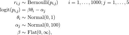
$r_{i,j} &\sim \text{Bernoulli}(p_{i,j}) \quad\quad i=1,\ldots,1000; j=1,\ldots,5 \\ \operatorname{logit}(p_{i,j}) &= \beta \theta_i - \alpha_j \\ \theta_i &\sim \text{Normal}(0, 1) \\ \alpha_j &\sim \text{Normal}(0, 100) \\ \beta &\sim \text{Flat}(0, \infty),$

where $r_{i,j}$ is an indicator for correct response by student $i$ to questions $j$ .

Analysis Program¶

using Mamba

## Data
lsat = (Symbol => Any)[
  :culm =>
    [3, 9, 11, 22, 23, 24, 27, 31, 32, 40, 40, 56, 56, 59, 61, 76, 86, 115, 129,
     210, 213, 241, 256, 336, 352, 408, 429, 602, 613, 674, 702, 1000],
  :response =>
    [0 0 0 0 0
     0 0 0 0 1
     0 0 0 1 0
     0 0 0 1 1
     0 0 1 0 0
     0 0 1 0 1
     0 0 1 1 0
     0 0 1 1 1
     0 1 0 0 0
     0 1 0 0 1
     0 1 0 1 0
     0 1 0 1 1
     0 1 1 0 0
     0 1 1 0 1
     0 1 1 1 0
     0 1 1 1 1
     1 0 0 0 0
     1 0 0 0 1
     1 0 0 1 0
     1 0 0 1 1
     1 0 1 0 0
     1 0 1 0 1
     1 0 1 1 0
     1 0 1 1 1
     1 1 0 0 0
     1 1 0 0 1
     1 1 0 1 0
     1 1 0 1 1
     1 1 1 0 0
     1 1 1 0 1
     1 1 1 1 0
     1 1 1 1 1],
  :N => 1000
]
lsat[:R] = size(lsat[:response], 1)
lsat[:T] = size(lsat[:response], 2)

n = [lsat[:culm][1], diff(lsat[:culm])]
idx = mapreduce(i -> fill(i, n[i]), vcat, 1:length(n))
lsat[:r] = lsat[:response][idx,:]


## Model Specification

model = Model(

  r = Stochastic(2,
    @modelexpr(beta, theta, alpha, N, T,
      Distribution[
        begin
          p = invlogit(beta * theta[i] - alpha[j])
          Bernoulli(p)
        end
        for i in 1:N, j in 1:T
      ]
    ),
    false
  ),

  theta = Stochastic(1,
    :(Normal(0, 1)),
    false
  ),

  alpha = Stochastic(1,
    :(Normal(0, 100)),
    false
  ),

  a = Logical(1,
    @modelexpr(alpha,
      alpha - mean(alpha)
    )
  ),

  beta = Stochastic(
    :(Truncated(Flat(), 0, Inf))
  )

)


## Initial Values
inits = [
  [:r => lsat[:r], :alpha => zeros(lsat[:T]), :beta => 1,
   :theta => zeros(lsat[:N])],
  [:r => lsat[:r], :alpha => ones(lsat[:T]), :beta => 2,
   :theta => zeros(lsat[:N])]
]


## Sampling Scheme
scheme = [AMWG([:alpha], fill(0.1, lsat[:T])),
          Slice([:beta], [1.0]),
          Slice([:theta], fill(0.5, lsat[:N]))]
setsamplers!(model, scheme)


## MCMC Simulations
sim = mcmc(model, lsat, inits, 10000, burnin=2500, thin=2, chains=2)
describe(sim)

Results¶

Iterations = 2502:10000
Thinning interval = 2
Chains = 1,2
Samples per chain = 3750

Empirical Posterior Estimates:
        Mean        SD      Naive SE        MCSE        ESS
a[1] -1.2631137 0.1050811 0.0012133719 0.00222282916 2234.791
a[2]  0.4781765 0.0690242 0.0007970227 0.00126502181 2977.191
a[3]  1.2401762 0.0679403 0.0007845071 0.00155219697 1915.850
a[4]  0.1705201 0.0716647 0.0008275129 0.00146377676 2396.962
a[5] -0.6257592 0.0858278 0.0009910540 0.00156546941 3005.846
beta  0.7648299 0.0567109 0.0006548411 0.00277090485  418.880

Quantiles:
        2.5%       25.0%     50.0%      75.0%      97.5%
a[1] -1.4797642 -1.3325895 -1.262183 -1.1898184 -1.0647215
a[2]  0.3493393  0.4300223  0.477481  0.5253468  0.6143681
a[3]  1.1090783  1.1936967  1.240509  1.2865947  1.3699112
a[4]  0.0285454  0.1221579  0.170171  0.2191623  0.3100302
a[5] -0.7970834 -0.6828463 -0.625013 -0.5685627 -0.4590098
beta  0.6618355  0.7249738  0.761457  0.8013506  0.8839082