Oxford: Smooth Fit to Log-Odds Ratios¶

An example from OpenBUGS [38] and Breslow and Clayton [9] concerning the association between death from childhood cancer and maternal exposure to X-rays, for subjects partitioned into 120 age and birth-year strata.

Model¶

Deaths are modelled as

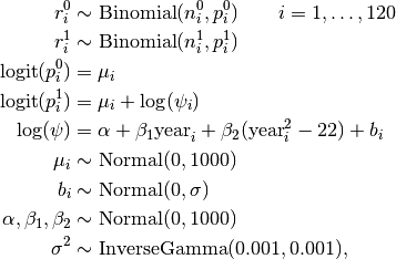
$r^0_i &\sim \text{Binomial}(n^0_i, p^0_i) \quad\quad i=1,\ldots,120 \\ r^1_i &\sim \text{Binomial}(n^1_i, p^1_i) \\ \operatorname{logit}(p^0_i) &= \mu_i \\ \operatorname{logit}(p^1_i) &= \mu_i + \log(\psi_i) \\ \log(\psi) &= \alpha + \beta_1 \text{year}_i + \beta_2 (\text{year}^2_i - 22) + b_i \\ \mu_i &\sim \text{Normal}(0, 1000) \\ b_i &\sim \text{Normal}(0, \sigma) \\ \alpha, \beta_1, \beta_2 &\sim \text{Normal}(0, 1000) \\ \sigma^2 &\sim \text{InverseGamma}(0.001, 0.001),$

where $r^0_i$ is the number of deaths among unexposed subjects in stratum $i$ , $r^1_i$ is the number among exposed subjects, and $\text{year}_i$ is the stratum-specific birth year (relative to 1954).

Analysis Program¶

using Mamba

## Data
oxford = (Symbol=> Any)[
  :r1 =>
    [3, 5, 2, 7, 7, 2, 5, 3, 5, 11, 6, 6, 11, 4, 4, 2, 8, 8, 6, 5, 15, 4, 9, 9,
     4, 12, 8, 8, 6, 8, 12, 4, 7, 16, 12, 9, 4, 7, 8, 11, 5, 12, 8, 17, 9, 3, 2,
     7, 6, 5, 11, 14, 13, 8, 6, 4, 8, 4, 8, 7, 15, 15, 9, 9, 5, 6, 3, 9, 12, 14,
     16, 17, 8, 8, 9, 5, 9, 11, 6, 14, 21, 16, 6, 9, 8, 9, 8, 4, 11, 11, 6, 9,
     4, 4, 9, 9, 10, 14, 6, 3, 4, 6, 10, 4, 3, 3, 10, 4, 10, 5, 4, 3, 13, 1, 7,
     5, 7, 6, 3, 7],
  :n1 =>
    [28, 21, 32, 35, 35, 38, 30, 43, 49, 53, 31, 35, 46, 53, 61, 40, 29, 44, 52,
     55, 61, 31, 48, 44, 42, 53, 56, 71, 43, 43, 43, 40, 44, 70, 75, 71, 37, 31,
     42, 46, 47, 55, 63, 91, 43, 39, 35, 32, 53, 49, 75, 64, 69, 64, 49, 29, 40,
     27, 48, 43, 61, 77, 55, 60, 46, 28, 33, 32, 46, 57, 56, 78, 58, 52, 31, 28,
     46, 42, 45, 63, 71, 69, 43, 50, 31, 34, 54, 46, 58, 62, 52, 41, 34, 52, 63,
     59, 88, 62, 47, 53, 57, 74, 68, 61, 45, 45, 62, 73, 53, 39, 45, 51, 55, 41,
     53, 51, 42, 46, 54, 32],
  :r0 =>
    [0, 2, 2, 1, 2, 0, 1, 1, 1, 2, 4, 4, 2, 1, 7, 4, 3, 5, 3, 2, 4, 1, 4, 5, 2,
     7, 5, 8, 2, 3, 5, 4, 1, 6, 5, 11, 5, 2, 5, 8, 5, 6, 6, 10, 7, 5, 5, 2, 8,
     1, 13, 9, 11, 9, 4, 4, 8, 6, 8, 6, 8, 14, 6, 5, 5, 2, 4, 2, 9, 5, 6, 7, 5,
     10, 3, 2, 1, 7, 9, 13, 9, 11, 4, 8, 2, 3, 7, 4, 7, 5, 6, 6, 5, 6, 9, 7, 7,
     7, 4, 2, 3, 4, 10, 3, 4, 2, 10, 5, 4, 5, 4, 6, 5, 3, 2, 2, 4, 6, 4, 1],
  :n0 =>
    [28, 21, 32, 35, 35, 38, 30, 43, 49, 53, 31, 35, 46, 53, 61, 40, 29, 44, 52,
     55, 61, 31, 48, 44, 42, 53, 56, 71, 43, 43, 43, 40, 44, 70, 75, 71, 37, 31,
     42, 46, 47, 55, 63, 91, 43, 39, 35, 32, 53, 49, 75, 64, 69, 64, 49, 29, 40,
     27, 48, 43, 61, 77, 55, 60, 46, 28, 33, 32, 46, 57, 56, 78, 58, 52, 31, 28,
     46, 42, 45, 63, 71, 69, 43, 50, 31, 34, 54, 46, 58, 62, 52, 41, 34, 52, 63,
     59, 88, 62, 47, 53, 57, 74, 68, 61, 45, 45, 62, 73, 53, 39, 45, 51, 55, 41,
     53, 51, 42, 46, 54, 32],
  :year =>
    [-10, -9, -9, -8, -8, -8, -7, -7, -7, -7, -6, -6, -6, -6, -6, -5, -5, -5,
     -5, -5, -5, -4, -4, -4, -4, -4, -4, -4, -3, -3, -3, -3, -3, -3, -3, -3, -2,
     -2, -2, -2, -2, -2, -2, -2, -2, -1, -1, -1, -1, -1, -1, -1, -1, -1, -1, 0,
     0, 0, 0, 0, 0, 0, 0, 0, 0, 1, 1, 1, 1, 1, 1, 1, 1, 1, 1, 2, 2, 2, 2, 2, 2,
     2, 2, 2, 3, 3, 3, 3, 3, 3, 3, 3, 4, 4, 4, 4, 4, 4, 4, 5, 5, 5, 5, 5, 5, 6,
     6, 6, 6, 6, 7, 7, 7, 7, 8, 8, 8, 9, 9, 10],
  :K => 120
]
oxford[:K] = length(oxford[:r1])


## Model Specification

model = Model(

  r0 = Stochastic(1,
    @modelexpr(mu, n0, K,
      begin
        p = invlogit(mu)
        Distribution[Binomial(n0[i], p[i]) for i in 1:K]
      end
    ),
    false
  ),

  r1 = Stochastic(1,
    @modelexpr(mu, alpha, beta1, beta2, year, b, n1, K,
      Distribution[
        begin
          p = invlogit(mu[i] + alpha + beta1 * year[i] +
                       beta2 * (year[i]^2 - 22.0) + b[i])
          Binomial(n1[i], p)
        end
        for i in 1:K
      ]
    ),
    false
  ),

  b = Stochastic(1,
    @modelexpr(s2,
      Normal(0, sqrt(s2))
    ),
    false
  ),

  mu = Stochastic(1,
    :(Normal(0, 1000)),
    false
  ),

  alpha = Stochastic(
    :(Normal(0, 1000))
  ),

  beta1 = Stochastic(
    :(Normal(0, 1000))
  ),

  beta2 = Stochastic(
    :(Normal(0, 1000))
  ),

  s2 = Stochastic(
    :(InverseGamma(0.001, 0.001))
  )

)


## Initial Values
inits = [
  [:r0 => oxford[:r0], :r1 => oxford[:r1], :alpha => 0, :beta1 => 0,
   :beta2 => 0, :s2 => 1, :b => zeros(oxford[:K]), :mu => zeros(oxford[:K])],
  [:r0 => oxford[:r0], :r1 => oxford[:r1], :alpha => 1, :beta1 => 1,
   :beta2 => 1, :s2 => 10, :b => zeros(oxford[:K]), :mu => zeros(oxford[:K])]
]


## Sampling Scheme
scheme = [AMWG([:alpha, :beta1, :beta2], fill(1.0, 3)),
          Slice([:s2], [1.0]),
          Slice([:mu], ones(oxford[:K])),
          Slice([:b], ones(oxford[:K]))]
setsamplers!(model, scheme)


## MCMC Simulations
sim = mcmc(model, oxford, inits, 12500, burnin=2500, thin=2, chains=2)
describe(sim)

Results¶

Iterations = 2502:12500
Thinning interval = 2
Chains = 1,2
Samples per chain = 5000

Empirical Posterior Estimates:
         Mean         SD        Naive SE       MCSE        ESS
alpha  0.5657848 0.063005090 0.00063005090 0.0034007318 343.24680
   s2  0.0262390 0.030798915 0.00030798915 0.0026076857 139.49555
beta1 -0.0433363 0.016175426 0.00016175426 0.0011077969 213.20196
beta2  0.0054771 0.003567575 0.00003567575 0.0002358424 228.82453

Quantiles:
          2.5%       25.0%      50.0%      75.0%       97.5%
alpha  0.44382579  0.5238801  0.5675039  0.60514271  0.6959681
   s2  0.00071344  0.0033353  0.0146737  0.03971325  0.1182023
beta1 -0.07451524 -0.0543180 -0.0434426 -0.03212161 -0.0099208
beta2 -0.00104990  0.0028489  0.0056500  0.00774736  0.0136309