Pumps: Gamma-Poisson Hierarchical Model¶

An example from OpenBUGS [38] and George et al. [32] concerning the number of failures of 10 power plant pumps.

Model¶

Pump failure are modelled as

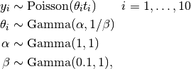
$y_i &\sim \text{Poisson}(\theta_i t_i) \quad\quad i=1,\ldots,10 \\ \theta_i &\sim \text{Gamma}(\alpha, 1 / \beta) \\ \alpha &\sim \text{Gamma}(1, 1) \\ \beta &\sim \text{Gamma}(0.1, 1),$

where $y_i$ is the number of times that pump $i$ failed, and $t_i$ is the operation time of the pump (in 1000s of hours).

Analysis Program¶

using Mamba

## Data
pumps = (Symbol => Any)[
  :y => [5, 1, 5, 14, 3, 19, 1, 1, 4, 22],
  :t => [94.3, 15.7, 62.9, 126, 5.24, 31.4, 1.05, 1.05, 2.1, 10.5]
]
pumps[:N] = length(pumps[:y])


## Model Specification

model = Model(

  y = Stochastic(1,
    @modelexpr(theta, t, N,
      Distribution[
        begin
          lambda = theta[i] * t[i]
          Poisson(lambda)
        end
        for i in 1:N
      ]
    ),
    false
  ),

  theta = Stochastic(1,
    @modelexpr(alpha, beta,
      Gamma(alpha, 1 / beta)
    ),
    true
  ),

  alpha = Stochastic(
    :(Exponential(1.0))
  ),

  beta = Stochastic(
    :(Gamma(0.1, 1.0))
  )

)


## Initial Values
inits = [
  [:y => pumps[:y], :alpha => 1.0, :beta => 1.0,
   :theta => rand(Gamma(1.0, 1.0), pumps[:N])],
  [:y => pumps[:y], :alpha => 10.0, :beta => 10.0,
   :theta => rand(Gamma(10.0, 10.0), pumps[:N])]
]


## Sampling Scheme
scheme = [Slice([:alpha, :beta], [1.0, 1.0], :univar),
          Slice([:theta], ones(pumps[:N]), :univar)]
setsamplers!(model, scheme)


## MCMC Simulations
sim = mcmc(model, pumps, inits, 10000, burnin=2500, thin=2, chains=2)
describe(sim)


## Posterior Predictive Distribution
ppd = predict(sim, :y)
describe(ppd)

Results¶

## MCMC Simulations

Iterations = 2502:10000
Thinning interval = 2
Chains = 1,2
Samples per chain = 3750

Empirical Posterior Estimates:
            Mean       SD       Naive SE      MCSE       ESS
 theta[1] 0.059728 0.02511183 0.000289966 0.000357021 4947.3086
 theta[2] 0.099763 0.07733395 0.000892976 0.001131733 4669.3099
 theta[3] 0.088984 0.03795487 0.000438265 0.000510879 5519.5005
 theta[4] 0.116179 0.03056397 0.000352922 0.000382914 6371.1555
 theta[5] 0.603654 0.32235984 0.003722291 0.006123252 2771.5172
 theta[6] 0.608916 0.13940546 0.001609716 0.001556592 7500.0000
 theta[7] 0.894307 0.69157282 0.007985595 0.030109699  527.5492
 theta[8] 0.884304 0.72603888 0.008383575 0.025229264  828.1530
 theta[9] 1.562347 0.75587826 0.008728130 0.023807874 1008.0045
theta[10] 1.987852 0.42786838 0.004940598 0.010220427 1752.5979
    alpha 0.679247 0.26700149 0.003083068 0.007082723 1421.1072
     beta 0.893892 0.52823112 0.006099488 0.018254904  837.3150

Quantiles:
             2.5%     25.0%     50.0%     75.0%     97.5%
 theta[1] 0.0210364 0.0413043 0.0561389 0.0742908 0.117973
 theta[2] 0.0077032 0.0433944 0.0812108 0.1359765 0.296096
 theta[3] 0.0309151 0.0616544 0.0841478 0.1106976 0.178913
 theta[4] 0.0635652 0.0944482 0.1137455 0.1351764 0.182949
 theta[5] 0.1481702 0.3696211 0.5496033 0.7757793 1.380921
 theta[6] 0.3666778 0.5100374 0.5997593 0.6959183 0.915158
 theta[7] 0.0781523 0.3743788 0.7229133 1.2273922 2.689196
 theta[8] 0.0734788 0.3736729 0.6900152 1.1995264 2.729814
 theta[9] 0.4625337 1.0045124 1.4399533 1.9909942 3.359561
theta[10] 1.2345761 1.6807668 1.9568796 2.2550151 2.907759
    alpha 0.2785980 0.4856731 0.6407352 0.8256277 1.324442
     beta 0.1770170 0.5026369 0.7839917 1.1795453 2.199956

## Posterior Predictive Distribution

Iterations = 2502:10000
Thinning interval = 2
Chains = 1,2
Samples per chain = 3750

Empirical Posterior Estimates:
         Mean      SD    Naive SE     MCSE       ESS
 y[1]  5.668000 3.41520 0.03943534 0.04402538 6017.6410
 y[2]  1.533467 1.70394 0.01967537 0.02404013 5023.8127
 y[3]  5.568533 3.38075 0.03903758 0.04069074 6902.9658
 y[4] 14.647333 5.45170 0.06295083 0.06597961 6827.2327
 y[5]  3.176400 2.46365 0.02844775 0.03740773 4337.4491
 y[6] 19.165467 6.20492 0.07164830 0.06647720 7500.0000
 y[7]  0.938400 1.20349 0.01389676 0.03474854 1199.5408
 y[8]  0.937200 1.22294 0.01412133 0.02790754 1920.2997
 y[9]  3.289333 2.39193 0.02761960 0.05164792 2144.8171
y[10] 20.863467 6.39303 0.07382033 0.11124836 3302.3719

Quantiles:
      2.5% 25.0% 50.0% 75.0% 97.5%
 y[1]    1     3     5     8    14
 y[2]    0     0     1     2     6
 y[3]    1     3     5     7    14
 y[4]    5    11    14    18    26
 y[5]    0     1     3     4     9
 y[6]    9    15    19    23    33
 y[7]    0     0     1     1     4
 y[8]    0     0     1     1     4
 y[9]    0     2     3     5     9
y[10]   10    16    20    25    35