Seeds: Random Effect Logistic Regression¶

An example from OpenBUGS [38], Crowder [17], and Breslow and Clayton [9] concerning the proportion of seeds that germinated on each of 21 plates arranged according to a 2 by 2 factorial layout by seed and type of root extract.

Model¶

Germinations are modelled as

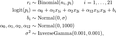
$r_i &\sim \text{Binomial}(n_i, p_i) \quad\quad i=1,\ldots,21 \\ \operatorname{logit}(p_i) &= \alpha_0 + \alpha_1 x_{1i} + \alpha_2 x_{2i} + \alpha_{12} x_{1i} x_{2i} + b_i \\ b_i &\sim \text{Normal}(0, \sigma) \\ \alpha_0, \alpha_1, \alpha_2, \alpha_{12} &\sim \text{Normal}(0, 1000) \\ \sigma^2 &\sim \text{InverseGamma}(0.001, 0.001),$

where $r_i$ are the number of seeds, out of $n_i$ , that germinate on plate $i$ ; and $x_{1i}$ and $x_{2i}$ are the seed type and root extract.

Analysis Program¶

using Mamba

## Data
seeds = (Symbol => Any)[
  :r => [10, 23, 23, 26, 17, 5, 53, 55, 32, 46, 10, 8, 10, 8, 23, 0, 3, 22, 15,
         32, 3],
  :n => [39, 62, 81, 51, 39, 6, 74, 72, 51, 79, 13, 16, 30, 28, 45, 4, 12, 41,
         30, 51, 7],
  :x1 => [0, 0, 0, 0, 0, 0, 0, 0, 0, 0, 0, 1, 1, 1, 1, 1, 1, 1, 1, 1, 1],
  :x2 => [0, 0, 0, 0, 0, 1, 1, 1, 1, 1, 1, 0, 0, 0, 0, 0, 1, 1, 1, 1, 1]
]
seeds[:N] = length(seeds[:r])


## Model Specification

model = Model(

  r = Stochastic(1,
    @modelexpr(alpha0, alpha1, x1, alpha2, x2, alpha12, b, n, N,
      Distribution[
        begin
          p = invlogit(alpha0 + alpha1 * x1[i] + alpha2 * x2[i] +
                       alpha12 * x1[i] * x2[i] + b[i])
          Binomial(n[i], p)
        end
        for i in 1:N
      ]
    ),
    false
  ),

  b = Stochastic(1,
    @modelexpr(s2,
      Normal(0, sqrt(s2))
    ),
    false
  ),

  alpha0 = Stochastic(
    :(Normal(0, 1000))
  ),

  alpha1 = Stochastic(
    :(Normal(0, 1000))
  ),

  alpha2 = Stochastic(
    :(Normal(0, 1000))
  ),

  alpha12 = Stochastic(
    :(Normal(0, 1000))
  ),

  s2 = Stochastic(
    :(InverseGamma(0.001, 0.001))
  )

)


## Initial Values
inits = [
  [:r => seeds[:r], :alpha0 => 0, :alpha1 => 0, :alpha2 => 0,
   :alpha12 => 0, :s2 => 0.01, :b => zeros(seeds[:N])],
  [:r => seeds[:r], :alpha0 => 0, :alpha1 => 0, :alpha2 => 0,
   :alpha12 => 0, :s2 => 1, :b => zeros(seeds[:N])]
]


## Sampling Scheme
scheme = [AMM([:alpha0, :alpha1, :alpha2, :alpha12], 0.01 * eye(4)),
          AMWG([:b], fill(0.01, seeds[:N])),
          AMWG([:s2], [0.1])]
setsamplers!(model, scheme)


## MCMC Simulations
sim = mcmc(model, seeds, inits, 12500, burnin=2500, thin=2, chains=2)
describe(sim)

Results¶

Iterations = 2502:12500
Thinning interval = 2
Chains = 1,2
Samples per chain = 5000

Empirical Posterior Estimates:
           Mean        SD       Naive SE       MCSE       ESS
 alpha2  1.3107281 0.26053104 0.0026053104 0.016391301 252.63418
     s2  0.0857053 0.09738014 0.0009738014 0.008167153 142.16720
 alpha0 -0.5561543 0.17595432 0.0017595432 0.011366011 239.65346
alpha12 -0.7464409 0.43006756 0.0043006756 0.026796428 257.58440
 alpha1  0.0887002 0.26872879 0.0026872879 0.013771345 380.78132

Quantiles:
            2.5%       25.0%      50.0%      75.0%      97.5%
 alpha2  0.80405938  1.1488818  1.3099477  1.4807632  1.8281561
     s2  0.00117398  0.0211176  0.0593763  0.1114008  0.3523464
 alpha0 -0.91491978 -0.6666323 -0.5512929 -0.4426242 -0.2224477
alpha12 -1.54570414 -1.0275765 -0.7572503 -0.4914919  0.1702970
 alpha1 -0.42501648 -0.0936379  0.0943906  0.2600758  0.6235393