Birats: A Bivariate Normal Hierarchical Model
An example from OpenBUGS [41] and section 6 of Gelfand et al. [27] concerning 30 rats whose weights were measured at each of five consecutive weeks.
Model
Weights are modeled as
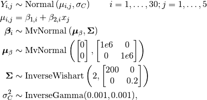
where  is repeated weight measurement
  on rat
  , and
, and  is the day on which the measurement was taken.
Analysis Program
using Mamba

## Data
birats = Dict{Symbol, Any}(
  :N => 30, :T => 5,
  :x => [8.0, 15.0, 22.0, 29.0, 36.0],
  :Y => [151 199 246 283 320
         145 199 249 293 354
         147 214 263 312 328
         155 200 237 272 297
         135 188 230 280 323
         159 210 252 298 331
         141 189 231 275 305
         159 201 248 297 338
         177 236 285 350 376
         134 182 220 260 296
         160 208 261 313 352
         143 188 220 273 314
         154 200 244 289 325
         171 221 270 326 358
         163 216 242 281 312
         160 207 248 288 324
         142 187 234 280 316
         156 203 243 283 317
         157 212 259 307 336
         152 203 246 286 321
         154 205 253 298 334
         139 190 225 267 302
         146 191 229 272 302
         157 211 250 285 323
         132 185 237 286 331
         160 207 257 303 345
         169 216 261 295 333
         157 205 248 289 316
         137 180 219 258 291
         153 200 244 286 324],
  :mean => [0.0, 0.0],
  :var => [1.0e6 0.0
           0.0   1.0e6],
  :Omega => [200.0 0.0
               0.0 0.2]
)


## Model Specification
model = Model(

  Y = Stochastic(2,
    (beta, x, sigmaC, N, T) ->
      UnivariateDistribution[
        Normal(beta[i, 1] + beta[i, 2] * x[j], sigmaC)
        for i in 1:N, j in 1:T
      ],
    false
  ),

  beta = Stochastic(2,
    (mu_beta, Sigma, N) ->
      MultivariateDistribution[
        MvNormal(mu_beta, Sigma)
        for i in 1:N
      ],
    false
  ),

  mu_beta = Stochastic(1,
    (mean, var) -> MvNormal(mean, var)
  ),

  Sigma = Stochastic(2,
    Omega -> InverseWishart(2, Omega),
    false
  ),

  sigma2C = Stochastic(
    () -> InverseGamma(0.001, 0.001),
    false
  ),

  sigmaC = Logical(
    sigma2C -> sqrt(sigma2C)
  )

)


## Initial Values
inits = [
  Dict(:Y => birats[:Y], :beta => repmat([100 6], birats[:N], 1),
       :mu_beta => [0, 0], :Sigma => eye(2), :sigma2C => 1.0),
  Dict(:Y => birats[:Y], :beta => repmat([50 3], birats[:N], 1),
       :mu_beta => [10, 10], :Sigma => 0.3 * eye(2), :sigma2C => 10.0)
]


## Sampling Scheme
scheme = [AMWG([:beta, :mu_beta], repmat([10.0, 1.0], birats[:N] + 1)),
          AMWG(:Sigma, 1.0),
          Slice(:sigma2C, 10.0)]
setsamplers!(model, scheme)


## MCMC Simulations
sim = mcmc(model, birats, inits, 10000, burnin=2500, thin=2, chains=2)
describe(sim)
Results
Iterations = 2502:10000
Thinning interval = 2
Chains = 1,2
Samples per chain = 3750

Empirical Posterior Estimates:
               Mean         SD       Naive SE       MCSE       ESS
mu_beta[1] 106.7046188 2.258246468 0.0260759841 0.081338282 770.81949
mu_beta[2]   6.1804557 0.104047928 0.0012014420 0.004102793 643.14317
    sigmaC   6.1431758 0.460583341 0.0053183583 0.021005830 480.76933

Quantiles:
               2.5%       25.0%       50.0%       75.0%      97.5%
mu_beta[1] 102.3595659 105.2252185 106.6914834 108.164852 111.2001520
mu_beta[2]   5.9720904   6.1130035   6.1817455   6.248025   6.3848798
    sigmaC   5.3167022   5.8123935   6.1206859   6.445419   7.0971249