Dyes: Variance Components Model¶

An example from OpenBUGS [41], Davies [19], and Box and Tiao [7] concerning batch-to-batch variation in yields from six batches and five samples of dyestuff.

Model¶

Yields are modelled as

$y_{i,j} &\sim \text{Normal}(\mu_i, \sigma_\text{within}) \quad\quad i=1,\ldots,6; j=1,\ldots,5 \\ \mu_i &\sim \text{Normal}(\theta, \sigma_\text{between}) \\ \theta &\sim \text{Normal}(0, 1000) \\ \sigma^2_\text{within}, \sigma^2_\text{between} &\sim \text{InverseGamma}(0.001, 0.001),$

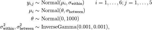
where $y_{i,j}$ is the response for batch $i$ and sample $j$ .

Analysis Program¶

using Mamba

## Data
dyes = Dict{Symbol, Any}(
  :y =>
    [1545, 1440, 1440, 1520, 1580,
     1540, 1555, 1490, 1560, 1495,
     1595, 1550, 1605, 1510, 1560,
     1445, 1440, 1595, 1465, 1545,
     1595, 1630, 1515, 1635, 1625,
     1520, 1455, 1450, 1480, 1445],
  :batches => 6,
  :samples => 5
)

dyes[:batch] = vcat([fill(i, dyes[:samples]) for i in 1:dyes[:batches]]...)
dyes[:sample] = vcat(fill(collect(1:dyes[:samples]), dyes[:batches])...)


## Model Specification

model = Model(

  y = Stochastic(1,
    (mu, batch, s2_within) -> MvNormal(mu[batch], sqrt(s2_within)),
    false
  ),

  mu = Stochastic(1,
    (theta, batches, s2_between) -> Normal(theta, sqrt(s2_between))
  ),

  theta = Stochastic(
    () -> Normal(0, 1000)
  ),

  s2_within = Stochastic(
    () -> InverseGamma(0.001, 0.001)
  ),

  s2_between = Stochastic(
    () -> InverseGamma(0.001, 0.001)
  )

)


## Initial Values
inits = [
  Dict(:y => dyes[:y], :theta => 1500, :s2_within => 1, :s2_between => 1,
       :mu => fill(1500, dyes[:batches])),
  Dict(:y => dyes[:y], :theta => 3000, :s2_within => 10, :s2_between => 10,
       :mu => fill(3000, dyes[:batches]))
]


## Sampling Schemes
scheme = [NUTS([:mu, :theta]),
          Slice([:s2_within, :s2_between], 1000.0)]

scheme2 = [MALA(:theta, 50.0),
           MALA(:mu, 50.0, eye(dyes[:batches])),
           Slice([:s2_within, :s2_between], 1000.0)]

scheme3 = [HMC(:theta, 10.0, 5),
           HMC(:mu, 10.0, 5, eye(dyes[:batches])),
           Slice([:s2_within, :s2_between], 1000.0)]

scheme4 = [RWM(:theta, 50.0, proposal=Cosine),
           RWM(:mu, 50.0),
           Slice([:s2_within, :s2_between], 1000.0)]


## MCMC Simulations
setsamplers!(model, scheme)
sim = mcmc(model, dyes, inits, 10000, burnin=2500, thin=2, chains=2)
describe(sim)

setsamplers!(model, scheme2)
sim2 = mcmc(model, dyes, inits, 10000, burnin=2500, thin=2, chains=2)
describe(sim2)

setsamplers!(model, scheme3)
sim3 = mcmc(model, dyes, inits, 10000, burnin=2500, thin=2, chains=2)
describe(sim3)

setsamplers!(model, scheme4)
sim4 = mcmc(model, dyes, inits, 10000, burnin=2500, thin=2, chains=2)
describe(sim4)

Results¶

Iterations = 2502:10000
Thinning interval = 2
Chains = 1,2
Samples per chain = 3750

Empirical Posterior Estimates:
              Mean        SD       Naive SE      MCSE         ESS
s2_between 3192.2614 4456.129102 51.45494673 487.44961486   83.57109
     theta 1526.7186   24.549671  0.28347518   0.37724897 3750.00000
 s2_within 2887.5853 1075.174260 12.41504296  76.89117959  195.52607
     mu[1] 1511.4798   20.819711  0.24040531   0.52158448 1593.30921
     mu[2] 1527.9087   20.344151  0.23491402   0.30199960 3750.00000
     mu[3] 1552.6742   21.293738  0.24587891   0.70276515  918.08605
     mu[4] 1506.6440   21.349176  0.24651905   0.61821290 1192.57616
     mu[5] 1578.6636   25.512471  0.29459264   1.29216105  389.82685
     mu[6] 1487.1934   24.693967  0.28514137   1.23710390  398.44592

Quantiles:
              2.5%      25.0%     50.0%     75.0%        97.5%
s2_between  111.92351  815.9012 1651.4605 3269.5663 1.90261752x104
     theta 1475.08243 1513.5687 1527.1763 1540.0550 1.57444106x103
 s2_within 1566.61796 2160.3251 2654.9358 3324.8621 5.65161862x103
     mu[1] 1469.68693 1498.0985 1511.3084 1525.7344 1.55281296x103
     mu[2] 1486.15990 1514.8487 1527.6843 1541.2155 1.56770562x103
     mu[3] 1512.72912 1537.7046 1552.1976 1566.7188 1.59498301x103
     mu[4] 1463.91701 1492.3206 1506.9856 1521.3449 1.54854165x103
     mu[5] 1528.52480 1562.1831 1579.2515 1596.0167 1.62731017x103
     mu[6] 1440.27721 1470.7983 1486.1844 1502.9911 1.54464614x103