Surgical: Institutional Ranking¶

An example from OpenBUGS [41] concerning mortality rates in 12 hospitals performing cardiac surgery in infants.

Model¶

Number of deaths are modelled as

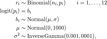
$r_i &\sim \text{Binomial}(n_i, p_i) \quad\quad i=1,\ldots,12 \\ \operatorname{logit}(p_i) &= b_i \\ b_i &\sim \text{Normal}(\mu, \sigma) \\ \mu &\sim \text{Normal}(0, 1000) \\ \sigma^2 &\sim \text{InverseGamma}(0.001, 0001),$

where $r_i$ is the number of deaths, out of $n_i$ operations, at hospital $i$ .

Analysis Program¶

using Mamba

## Data
surgical = Dict{Symbol, Any}(
  :r => [0, 18, 8, 46, 8, 13, 9, 31, 14, 8, 29, 24],
  :n => [47, 148, 119, 810, 211, 196, 148, 215, 207, 97, 256, 360]
)
surgical[:N] = length(surgical[:r])


## Model Specification
model = Model(

  r = Stochastic(1,
    (n, p, N) ->
      UnivariateDistribution[Binomial(n[i], p[i]) for i in 1:N],
    false
  ),

  p = Logical(1,
    b -> invlogit(b)
  ),

  b = Stochastic(1,
    (mu, s2) -> Normal(mu, sqrt(s2)),
    false
  ),

  mu = Stochastic(
    () -> Normal(0, 1000)
  ),

  pop_mean = Logical(
    mu -> invlogit(mu)
  ),

  s2 = Stochastic(
    () -> InverseGamma(0.001, 0.001)
  )

)

## Initial Values
inits = [
  Dict(:r => surgical[:r], :b => fill(0.1, surgical[:N]), :s2 => 1, :mu => 0),
  Dict(:r => surgical[:r], :b => fill(0.5, surgical[:N]), :s2 => 10, :mu => 1)
]


## Sampling Scheme
scheme = [NUTS(:b),
          Slice([:mu, :s2], 1.0)]
setsamplers!(model, scheme)


## MCMC Simulations
sim = mcmc(model, surgical, inits, 10000, burnin=2500, thin=2, chains=2)
describe(sim)

Results¶

Iterations = 2502:10000
Thinning interval = 2
Chains = 1,2
Samples per chain = 3750

Empirical Posterior Estimates:
             Mean          SD        Naive SE         MCSE        ESS
      mu -2.550263247 0.151813688 0.001752993476 0.00352027397 1859.8115
pop_mean  0.073062651 0.010097974 0.000116601357 0.00022880854 1947.7088
      s2  0.183080212 0.161182244 0.001861172237 0.00629499754  655.6065
    p[1]  0.053571675 0.019444542 0.000224526231 0.00059140521 1080.9986
    p[2]  0.103203725 0.022015796 0.000254216516 0.00049928289 1944.3544
    p[3]  0.071050270 0.017662050 0.000203943787 0.00022426787 3750.0000
    p[4]  0.059863573 0.008208359 0.000094781965 0.00033190971  611.6074
    p[5]  0.052400628 0.013632842 0.000157418497 0.00052344316  678.3186
    p[6]  0.069799258 0.014697820 0.000169715805 0.00026854081 2995.6099
    p[7]  0.066927057 0.015703466 0.000181328008 0.00023888938 3750.0000
    p[8]  0.122296440 0.023319424 0.000269269516 0.00086456417  727.5137
    p[9]  0.070386216 0.014318572 0.000165336624 0.00019674962 3750.0000
   p[10]  0.077978945 0.019775182 0.000228344129 0.00031544646 3750.0000
   p[11]  0.101809685 0.017568938 0.000202868617 0.00037809859 2159.1405
   p[12]  0.068534503 0.011579540 0.000133709009 0.00015162331 3750.0000

Quantiles:
             2.5%         25.0%        50.0%        75.0%        97.5%
      mu -2.878686485 -2.637983754 -2.540103608 -2.455828143 -2.269200544
pop_mean  0.053217279  0.066733498  0.073094153  0.079013392  0.093706084
      s2  0.011890649  0.082427721  0.141031919  0.233947847  0.601137558
    p[1]  0.017683165  0.039573948  0.052942713  0.067219732  0.092219913
    p[2]  0.067482073  0.086541186  0.100283541  0.116521584  0.153268132
    p[3]  0.040088134  0.059099562  0.070320337  0.080842394  0.110595078
    p[4]  0.044965780  0.054145641  0.059405801  0.065149564  0.076754218
    p[5]  0.028224773  0.042599948  0.051613569  0.061247876  0.079162530
    p[6]  0.043031618  0.059518315  0.069130011  0.079935035  0.100122661
    p[7]  0.038586653  0.055992241  0.066465865  0.076006492  0.101351899
    p[8]  0.082604334  0.105852706  0.121313052  0.137724088  0.171202438
    p[9]  0.044453383  0.060622475  0.070120723  0.079078759  0.101046045
   p[10]  0.044439834  0.064694148  0.075946776  0.089236114  0.122899027
   p[11]  0.071966143  0.088360531  0.100133691  0.112632331  0.139968412
   p[12]  0.047466661  0.060611827  0.068267225  0.075638053  0.093309250