LSAT: Item Response¶

An example from OpenBUGS [43] and Boch and Lieberman [6] concerning a 5-item multiple choice test (32 possible response patters) given to 1000 students.

Model¶

Item responses are modelled as

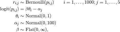
$r_{i,j} &\sim \text{Bernoulli}(p_{i,j}) \quad\quad i=1,\ldots,1000; j=1,\ldots,5 \\ \operatorname{logit}(p_{i,j}) &= \beta \theta_i - \alpha_j \\ \theta_i &\sim \text{Normal}(0, 1) \\ \alpha_j &\sim \text{Normal}(0, 100) \\ \beta &\sim \text{Flat}(0, \infty),$

where $r_{i,j}$ is an indicator for correct response by student $i$ to questions $j$ .

Analysis Program¶

using Mamba

## Data
lsat = Dict{Symbol, Any}(
  :culm =>
    [3, 9, 11, 22, 23, 24, 27, 31, 32, 40, 40, 56, 56, 59, 61, 76, 86, 115, 129,
     210, 213, 241, 256, 336, 352, 408, 429, 602, 613, 674, 702, 1000],
  :response =>
    [0 0 0 0 0
     0 0 0 0 1
     0 0 0 1 0
     0 0 0 1 1
     0 0 1 0 0
     0 0 1 0 1
     0 0 1 1 0
     0 0 1 1 1
     0 1 0 0 0
     0 1 0 0 1
     0 1 0 1 0
     0 1 0 1 1
     0 1 1 0 0
     0 1 1 0 1
     0 1 1 1 0
     0 1 1 1 1
     1 0 0 0 0
     1 0 0 0 1
     1 0 0 1 0
     1 0 0 1 1
     1 0 1 0 0
     1 0 1 0 1
     1 0 1 1 0
     1 0 1 1 1
     1 1 0 0 0
     1 1 0 0 1
     1 1 0 1 0
     1 1 0 1 1
     1 1 1 0 0
     1 1 1 0 1
     1 1 1 1 0
     1 1 1 1 1],
  :N => 1000
)
lsat[:R] = size(lsat[:response], 1)
lsat[:T] = size(lsat[:response], 2)

n = [lsat[:culm][1]; diff(lsat[:culm])]
idx = mapreduce(i -> fill(i, n[i]), vcat, 1:length(n))
lsat[:r] = lsat[:response][idx, :]


## Model Specification

model = Model(

  r = Stochastic(2,
    (beta, theta, alpha, N, T) ->
      UnivariateDistribution[
        begin
          p = invlogit(beta * theta[i] - alpha[j])
          Bernoulli(p)
        end
        for i in 1:N, j in 1:T
      ],
    false
  ),

  theta = Stochastic(1,
    () -> Normal(0, 1),
    false
  ),

  alpha = Stochastic(1,
    () -> Normal(0, 100),
    false
  ),

  a = Logical(1,
    alpha -> alpha - mean(alpha)
  ),

  beta = Stochastic(
    () -> Truncated(Flat(), 0, Inf)
  )

)


## Initial Values
inits = [
  Dict(:r => lsat[:r], :alpha => zeros(lsat[:T]), :beta => 1,
       :theta => zeros(lsat[:N])),
  Dict(:r => lsat[:r], :alpha => ones(lsat[:T]), :beta => 2,
       :theta => zeros(lsat[:N]))
]


## Sampling Scheme
scheme = [AMWG(:alpha, 0.1),
          Slice(:beta, 1.0),
          Slice(:theta, 0.5)]
setsamplers!(model, scheme)


## MCMC Simulations
sim = mcmc(model, lsat, inits, 10000, burnin=2500, thin=2, chains=2)
describe(sim)

Results¶

Iterations = 2502:10000
Thinning interval = 2
Chains = 1,2
Samples per chain = 3750

Empirical Posterior Estimates:
         Mean         SD        Naive SE       MCSE         ESS
beta  0.80404469 0.072990202 0.00084281825 0.0067491110  116.95963
a[1] -1.26236241 0.104040037 0.00120135087 0.0025355922 1683.61261
a[2]  0.48004293 0.069256031 0.00079969977 0.0013701533 2554.91753
a[3]  1.24206491 0.068338749 0.00078910790 0.0018426724 1375.42777
a[4]  0.16982672 0.072942222 0.00084226422 0.0012659899 3319.68982
a[5] -0.62957215 0.086601562 0.00099998871 0.0018787409 2124.79816

Quantiles:
         2.5%        25.0%       50.0%       75.0%       97.5%
beta  0.678005795  0.75195190  0.79754709  0.85100547  0.96030934
a[1] -1.471693755 -1.33040793 -1.25998457 -1.19317801 -1.06168159
a[2]  0.347262397  0.43161040  0.48023957  0.52718291  0.61527668
a[3]  1.106413529  1.19669095  1.24105794  1.28858225  1.37451854
a[4]  0.023253916  0.11970853  0.17099598  0.21998896  0.30858397
a[5] -0.799988061 -0.68755932 -0.63052599 -0.57168504 -0.46028931