Rats: A Normal Hierarchical Model

An example from OpenBUGS [43] and section 6 of Gelfand et al. [28] concerning 30 rats whose weights were measured at each of five consecutive weeks.

Model

Weights are modeled as

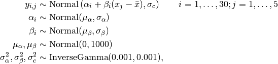
where is repeated weight measurement on rat , and is the day on which the measurement was taken.

Analysis Program

using Mamba

## Data
rats = Dict{Symbol, Any}(
  :y =>
    [151, 199, 246, 283, 320,
     145, 199, 249, 293, 354,
     147, 214, 263, 312, 328,
     155, 200, 237, 272, 297,
     135, 188, 230, 280, 323,
     159, 210, 252, 298, 331,
     141, 189, 231, 275, 305,
     159, 201, 248, 297, 338,
     177, 236, 285, 350, 376,
     134, 182, 220, 260, 296,
     160, 208, 261, 313, 352,
     143, 188, 220, 273, 314,
     154, 200, 244, 289, 325,
     171, 221, 270, 326, 358,
     163, 216, 242, 281, 312,
     160, 207, 248, 288, 324,
     142, 187, 234, 280, 316,
     156, 203, 243, 283, 317,
     157, 212, 259, 307, 336,
     152, 203, 246, 286, 321,
     154, 205, 253, 298, 334,
     139, 190, 225, 267, 302,
     146, 191, 229, 272, 302,
     157, 211, 250, 285, 323,
     132, 185, 237, 286, 331,
     160, 207, 257, 303, 345,
     169, 216, 261, 295, 333,
     157, 205, 248, 289, 316,
     137, 180, 219, 258, 291,
     153, 200, 244, 286, 324],
  :x => [8.0, 15.0, 22.0, 29.0, 36.0]
)
rats[:xbar] = mean(rats[:x])
rats[:N] = size(rats[:y], 1)
rats[:T] = size(rats[:y], 2)

rats[:rat] = Int[div(i - 1, 5) + 1 for i in 1:150]
rats[:week] = Int[(i - 1) % 5 + 1 for i in 1:150]
rats[:X] = rats[:x][rats[:week]]
rats[:Xm] = rats[:X] - rats[:xbar]


## Model Specification
model = Model(

  y = Stochastic(1,
    (alpha, beta, rat, Xm, s2_c) ->
      begin
        mu = alpha[rat] + beta[rat] .* Xm
        MvNormal(mu, sqrt(s2_c))
      end,
    false
  ),

  alpha = Stochastic(1,
    (mu_alpha, s2_alpha) -> Normal(mu_alpha, sqrt(s2_alpha)),
    false
  ),

  alpha0 = Logical(
    (mu_alpha, xbar, mu_beta) -> mu_alpha - xbar * mu_beta
  ),

  mu_alpha = Stochastic(
    () -> Normal(0.0, 1000),
    false
  ),

  s2_alpha = Stochastic(
    () -> InverseGamma(0.001, 0.001),
    false
  ),

  beta = Stochastic(1,
    (mu_beta, s2_beta) -> Normal(mu_beta, sqrt(s2_beta)),
    false
  ),

  mu_beta = Stochastic(
    () -> Normal(0.0, 1000)
  ),

  s2_beta = Stochastic(
    () -> InverseGamma(0.001, 0.001),
    false
  ),

  s2_c = Stochastic(
    () -> InverseGamma(0.001, 0.001)
  )

)


## Initial Values
inits = [
  Dict(:y => rats[:y], :alpha => fill(250, 30), :beta => fill(6, 30),
       :mu_alpha => 150, :mu_beta => 10, :s2_c => 1, :s2_alpha => 1,
       :s2_beta => 1),
  Dict(:y => rats[:y], :alpha => fill(20, 30), :beta => fill(0.6, 30),
       :mu_alpha => 15, :mu_beta => 1, :s2_c => 10, :s2_alpha => 10,
       :s2_beta => 10)
]


## Sampling Scheme
scheme = [Slice(:s2_c, 10.0),
          AMWG(:alpha, 100.0),
          Slice([:mu_alpha, :s2_alpha], [100.0, 10.0], Univariate),
          AMWG(:beta, 1.0),
          Slice([:mu_beta, :s2_beta], 1.0, Univariate)]
setsamplers!(model, scheme)


## MCMC Simulations
sim = mcmc(model, rats, inits, 10000, burnin=2500, thin=2, chains=2)
describe(sim)

Results

Iterations = 2502:10000
Thinning interval = 2
Chains = 1,2
Samples per chain = 3750

Empirical Posterior Estimates:
            Mean         SD       Naive SE       MCSE        ESS
   s2_c  37.2543133 6.026634572 0.0695895819 0.2337982327  664.4576
mu_beta   6.1830663 0.108042927 0.0012475723 0.0017921615 3634.4474
 alpha0 106.6259925 3.459210115 0.0399435178 0.0526804390 3750.0000

Quantiles:
           2.5%      25.0%       50.0%       75.0%       97.5%
   s2_c 27.778388  33.0906026  36.4630047  40.5538472  51.5713716
mu_beta  5.969850   6.1110307   6.1836454   6.2538831   6.3964953
 alpha0 99.815707 104.3369878 106.6105679 108.9124224 113.5045347