Tutorial
The complete source code for the examples contained in this tutorial can be obtained here.
Bayesian Linear Regression Model
In the sections that follow, the Bayesian simple linear regression example from the BUGS 0.5 manual [89] is used to illustrate features of the package. The example describes a regression relationship between observations  and
and  that can be expressed as
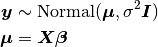
with prior distribution specifications
where 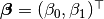 , and
, and  is a design matrix with an intercept vector of ones in the first column and
  in the second. Primary interest lies in making inference about the
  ,
,  , and
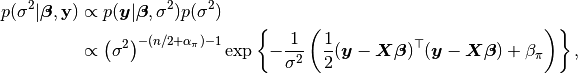
, and  parameters, based on their posterior distribution. A computational consideration in this example is that inference cannot be obtain from the joint posterior directly because of its nonstandard form, derived below up to a constant of proportionality.
A common alternative is to make approximate inference based on parameter values simulated from the posterior with MCMC methods.
Model Specification
Nodes
In the Mamba package, terms that appear in the Bayesian model specification are referred to as nodes. Nodes are classified as one of three types:
- Stochastic nodes are any model terms that have likelihood or prior distributional specifications. In the regression example,
,
, and
- Logical nodes are terms, like
, that are deterministic functions of other nodes.
- Input nodes are any remaining model terms (
Note that the node has both a distributional specification and is a fixed quantity. It is designated a stochastic node in Mamba because of its distributional specification. This allows for the possibility of model terms with distributional specifications that are a mix of observed and unobserved elements, as in the case of missing values in response vectors.
Model implementation begins by instantiating stochastic and logical nodes using the Mamba–supplied constructors Stochastic and Logical. Stochastic and logical nodes for a model are defined with a call to the Model constructor. The model constructor formally defines and assigns names to the nodes. User-specified names are given on the left-hand sides of the arguments to which Logical and Stochastic nodes are passed.
using Mamba, LinearAlgebra

## Model Specification

model = Model(

  y = Stochastic(1,
    (mu, s2) ->  MvNormal(mu, sqrt(s2)),
    false
  ),

  mu = Logical(1,
    (xmat, beta) -> xmat * beta,
    false
  ),

  beta = Stochastic(1,
    () -> MvNormal(2, sqrt(1000))
  ),

  s2 = Stochastic(
    () -> InverseGamma(0.001, 0.001)
  )

)
A single integer value for the first Stochastic constructor argument indicates that the node is an array of the specified dimension. Absence of an integer value implies a scalar node. The next argument is a function that may contain any valid julia code. Functions should be defined to take, as their arguments, the inputs upon which their nodes depend and, for stochastic nodes, return distribution objects or arrays of objects compatible with the Distributions package [2]. Such objects represent the nodes’ distributional specifications. An optional boolean argument after the function can be specified to indicate whether values of the node should be monitored (saved) during MCMC simulations (default: true).
Stochastic functions must return a single distribution object that can accommodate the dimensionality of the node, or return an array of (univariate or multivariate) distribution objects of the same dimension as the node. Examples of alternative, but equivalent, prior distributional specifications for the beta node are shown below.
# Case 1: Multivariate Normal with independence covariance matrix
beta = Stochastic(1,
  () -> MvNormal(2, sqrt(1000))
)

# Case 2: One common univariate Normal
beta = Stochastic(1,
  () -> Normal(0, sqrt(1000))
)

# Case 3: Array of univariate Normals
beta = Stochastic(1,
  () -> UnivariateDistribution[Normal(0, sqrt(1000)), Normal(0, sqrt(1000))]
)

# Case 4: Array of univariate Normals
beta = Stochastic(1,
  () -> UnivariateDistribution[Normal(0, sqrt(1000)) for i in 1:2]
)
Case 1 is one of the multivariate normal distributions available in the Distributions package, and the specification used in the example model implementation. In Case 2, a single univariate normal distribution is specified to imply independent priors of the same type for all elements of beta. Cases 3 and 4 explicitly specify a univariate prior for each element of beta and allow for the possibility of differences among the priors. Both return arrays of Distribution objects, with the last case automating the specification of array elements.
In summary, y and beta are stochastic vectors, s2 is a stochastic scalar, and mu is a logical vector. We note that the model could have been implemented without mu. It is included here primarily to illustrate use of a logical node. Finally, note that nodes y and mu are not being monitored.
Sampling Schemes
The package provides a flexible system for the specification of schemes to sample stochastic nodes. Arbitrary blocking of nodes and designation of block-specific samplers is supported. Furthermore, block-updating of nodes can be performed with samplers provided, defined by the user, or available from other packages. Schemes are specified as vectors of Sampler objects. Constructors are provided for several popular sampling algorithms, including adaptive Metropolis, No-U-Turn (NUTS), and slice sampling. Example schemes are shown below. In the first one, NUTS is used for the sampling of beta and slice for s2. The two nodes are block together in the second scheme and sampled jointly with NUTS.
## Hybrid No-U-Turn and Slice Sampling Scheme
scheme1 = [NUTS(:beta),
           Slice(:s2, 3.0)]

## No-U-Turn Sampling Scheme
scheme2 = [NUTS([:beta, :s2])]
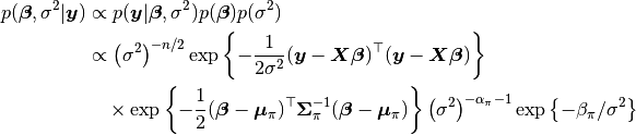
Additionally, users are free to create their own samplers with the generic Sampler constructor. This is particularly useful in settings were full conditional distributions are of standard forms for some nodes and can be sampled from directly. Such is the case for the full conditional of which can be written as
where  and
and 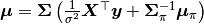 , and is recognizable as multivariate normal. Likewise,
whose form is inverse gamma with  shape and
  scale parameters. A user-defined sampling scheme to generate draws from these full conditionals is constructed below. Another example is given in the Pollution example for the sampling of multiple nodes.
## User-Defined Samplers
Gibbs_beta = Sampler([:beta],
(beta, s2, xmat, y) ->
begin
beta_mean = mean(beta.distr)
beta_invcov = invcov(beta.distr)
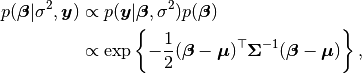
Sigma = inv(Symmetric(xmat' * xmat / s2 + beta_invcov))
mu = Sigma * (xmat' * y / s2 + beta_invcov * beta_mean)
rand(MvNormal(mu, Sigma))
end
)
Gibbs_s2 = Sampler([:s2],
(mu, s2, y) ->
begin
a = length(y) / 2.0 + shape(s2.distr)
b = sum(abs2, y - mu) / 2.0 + scale(s2.distr)
rand(InverseGamma(a, b))
end
)
## User-Defined Sampling Scheme
scheme3 = [Gibbs_beta, Gibbs_s2]
In these samplers, the respective MvNormal(2, sqrt(1000)) and InverseGamma(0.001, 0.001) priors on stochastic nodes beta and s2 are accessed directly through the distr fields. Features of the Distributions objects returned by beta.distr and s2.distr can, in turn, be extracted with method functions defined in that package or through their own fields. For instance, mean(beta.distr) and invcov(beta.distr) apply method functions to extract the mean vector and inverse-covariance matrix of the beta prior. Whereas, shape(s2.distr) and scale(s2.distr) extract the shape and scale parameters from fields of the inverse-gamma prior. Distributions method functions can be found in that package’s documentation; whereas, fields are found in the source code.
When possible to do so, direct sampling from full conditions is often preferred in practice because it tends to be more efficient than general-purpose algorithms. Schemes that mix the two approaches can be used if full conditionals are available for some model parameters but not for others. Once a sampling scheme is formulated in Mamba, it can be assigned to an existing model with a call to the setsamplers! function.
## Sampling Scheme Assignment
setsamplers!(model, scheme1)
Alternatively, a predefined scheme can be passed in to the Model constructor at the time of model implementation as the value to its samplers argument.
Directed Acyclic Graphs
One of the internal structures created by Model is a graph representation of the model nodes and their associations. Graphs are managed internally with the LightGraphs package [11]. Like OpenBUGS, JAGS, and other BUGS clones, Mamba fits models whose nodes form a directed acyclic graph (DAG). A DAG is a graph in which nodes are connected by directed edges and no node has a path that loops back to itself. With respect to statistical models, directed edges point from parent nodes to the child nodes that depend on them. Thus, a child node is independent of all others, given its parents.
The DAG representation of a Model can be printed out at the command-line or saved to an external file in a format that can be displayed with the Graphviz software.
## Graph Representation of Nodes

>>> draw(model)

digraph MambaModel {
  "mu" [shape="diamond", fillcolor="gray85", style="filled"];
    "mu" -> "y";
  "xmat" [shape="box", fillcolor="gray85", style="filled"];
    "xmat" -> "mu";
  "beta" [shape="ellipse"];
    "beta" -> "mu";
  "s2" [shape="ellipse"];
    "s2" -> "y";
  "y" [shape="ellipse", fillcolor="gray85", style="filled"];
}

>>> draw(model, filename="lineDAG.dot")
Either the printed or saved output can be passed manually to the Graphviz software to plot a visual representation of the model. If julia is being used with a front-end that supports in-line graphics, like IJulia [50], and the GraphViz julia package [26] is installed, then the following code will plot the graph automatically.
using GraphViz

>>> display(Graph(graph2dot(model)))
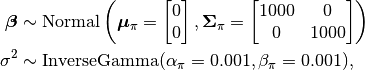
A generated plot of the regression model graph is show in the figure below.
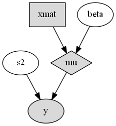
Directed acyclic graph representation of the example regression model nodes.
Stochastic, logical, and input nodes are represented by ellipses, diamonds, and rectangles, respectively. Gray-colored nodes are ones designated as unmonitored in MCMC simulations. The DAG not only allows the user to visually check that the model specification is the intended one, but is also used internally to check that nodal relationships are acyclic.
MCMC Simulation
Data
For the example, observations  are stored in a julia dictionary defined in the code block below. Included are predictor and response vectors
 :x and :y as well as a design matrix :xmat corresponding to the model matrix .
## Data
line = Dict{Symbol, Any}(
  :x => [1, 2, 3, 4, 5],
  :y => [1, 3, 3, 3, 5]
)
line[:xmat] = [ones(5) line[:x]]
Initial Values
A julia vector of dictionaries containing initial values for all stochastic nodes must be created. The dictionary keys should match the node names, and their values should be vectors whose elements are the same type of structures as the nodes. Three sets of initial values for the regression example are created in with the following code.
## Initial Values
inits = [
  Dict{Symbol, Any}(
    :y => line[:y],
    :beta => rand(Normal(0, 1), 2),
    :s2 => rand(Gamma(1, 1))
  )
for i in 1:3
]
Initial values for y are those in the observed response vector. Likewise, the node is not updated in the sampling schemes defined earlier and thus retains its initial values throughout MCMC simulations. Initial values are generated for beta from a normal distribution and for s2 from a gamma distribution.
MCMC Engine
MCMC simulation of draws from the posterior distribution of a declared set of model nodes and sampling scheme is performed with the mcmc() function. As shown below, the first three arguments are a Model object, a dictionary of values for input nodes, and a dictionary vector of initial values. The number of draws to generate in each simulation run is given as the fourth argument. The remaining arguments are named such that burnin is the number of initial values to discard to allow for convergence; thin defines the interval between draws to be retained in the output; and chains specifies the number of times to run the simulator. Results are returned as Chains objects on which methods for posterior inference are defined.
## MCMC Simulations

setsamplers!(model, scheme1)
sim1 = mcmc(model, line, inits, 10000, burnin=250, thin=2, chains=3)

setsamplers!(model, scheme2)
sim2 = mcmc(model, line, inits, 10000, burnin=250, thin=2, chains=3)

setsamplers!(model, scheme3)
sim3 = mcmc(model, line, inits, 10000, burnin=250, thin=2, chains=3)
Parallel Computing
The simulation of multiple chains will be executed in parallel automatically if julia is running in multiprocessor mode on a multiprocessor system. Multiprocessor mode can be started with the command line argument julia -p n, where n is the number of available processors. See the julia documentation on parallel computing for details.
Posterior Inference
Convergence Diagnostics
Checks of MCMC output should be performed to assess convergence of simulated draws to the posterior distribution. Checks can be performed with a variety of methods. The diagnostic of Gelman, Rubin, and Brooks [33][12] is one method for assessing convergence of posterior mean estimates. Values of the diagnostic’s potential scale reduction factor (PSRF) that are close to one suggest convergence. As a rule-of-thumb, convergence is rejected if the 97.5 percentile of a PSRF is greater than 1.2.
>>> gelmandiag(sim1, mpsrf=true, transform=true) |> showall

Gelman, Rubin, and Brooks Diagnostic:
              PSRF 97.5%
     beta[1] 1.009 1.010
     beta[2] 1.009 1.010
          s2 1.008 1.016
Multivariate 1.006   NaN
The diagnostic of Geweke [37] tests for non-convergence of posterior mean estimates. It provides chain-specific test p-values. Convergence is rejected for significant p-values, like those obtained for s2.
>>> gewekediag(sim1) |> showall

Geweke Diagnostic:
First Window Fraction = 0.1
Second Window Fraction = 0.5

        Z-score p-value
beta[1]   1.237  0.2162
beta[2]  -1.568  0.1168
     s2   1.710  0.0872

        Z-score p-value
beta[1]  -1.457  0.1452
beta[2]   1.752  0.0797
     s2  -1.428  0.1534

        Z-score p-value
beta[1]   0.550  0.5824
beta[2]  -0.440  0.6597
     s2   0.583  0.5596
The diagnostic of Heidelberger and Welch [47] tests for non-convergence (non-stationarity) and whether ratios of estimation interval halfwidths to means are within a target ratio. Stationarity is rejected (0) for significant test p-values. Halfwidth tests are rejected (0) if observed ratios are greater than the target, as is the case for s2 and beta[1].
>>> heideldiag(sim1) |> showall

Heidelberger and Welch Diagnostic:
Target Halfwidth Ratio = 0.1
Alpha = 0.05

        Burn-in Stationarity p-value    Mean     Halfwidth  Test
beta[1]     251            1  0.0680 0.57366275 0.053311283    1
beta[2]     738            1  0.0677 0.81285744 0.015404173    1
     s2     738            1  0.0700 1.00825202 0.094300432    1

        Burn-in Stationarity p-value    Mean     Halfwidth  Test
beta[1]     251            1  0.1356  0.6293320 0.065092099    0
beta[2]     251            1  0.0711  0.7934633 0.019215278    1
     s2     251            1  0.4435  1.4635400 0.588158612    0

        Burn-in Stationarity p-value    Mean     Halfwidth  Test
beta[1]     251            1  0.0515  0.5883602 0.058928034    0
beta[2]    1225            1  0.1479  0.8086080 0.018478999    1
     s2     251            1  0.6664  0.9942853 0.127959523    0
The diagnostic of Raftery and Lewis [74][75] is used to determine the number of iterations required to estimate a specified quantile within a desired degree of accuracy. For example, below are required total numbers of iterations, numbers to discard as burn-in sequences, and thinning intervals for estimating 0.025 quantiles so that their estimated cumulative probabilities are within 0.025±0.005 with probability 0.95.
>>> rafterydiag(sim1) |> showall

Raftery and Lewis Diagnostic:
Quantile (q) = 0.025
Accuracy (r) = 0.005
Probability (s) = 0.95

        Thinning Burn-in    Total   Nmin Dependence Factor
beta[1]        2     267      17897 3746         4.7776295
beta[2]        2     267      17897 3746         4.7776295
     s2        2     257       8689 3746         2.3195408

        Thinning Burn-in    Total   Nmin Dependence Factor
beta[1]        4     271 2.1759x10⁴ 3746         5.8085958
beta[2]        4     275 2.8795x10⁴ 3746         7.6868660
     s2        2     257 8.3450x10³ 3746         2.2277096

        Thinning Burn-in    Total   Nmin Dependence Factor
beta[1]        2     269 2.0647x10⁴ 3746         5.5117459
beta[2]        2     263 1.4523x10⁴ 3746         3.8769354
     s2        2     255 7.8770x10³ 3746         2.1027763
More information on the diagnostic functions can be found in the Convergence Diagnostics section.
Posterior Summaries
Once convergence has been assessed, sample statistics may be computed on the MCMC output to estimate features of the posterior distribution. The StatsBase package [53] is utilized in the calculation of many posterior estimates. Some of the available posterior summaries are illustrated in the code block below.
## Summary Statistics
>>> describe(sim1)

Iterations = 252:10000
Thinning interval = 2
Chains = 1,2,3
Samples per chain = 4875

Empirical Posterior Estimates:
           Mean       SD       Naive SE       MCSE       ESS
beta[1] 0.5971183 1.14894446 0.0095006014 0.016925598 4607.9743
beta[2] 0.8017036 0.34632566 0.0028637608 0.004793345 4875.0000
     s2 1.2203777 2.00876760 0.0166104638 0.101798287  389.3843

Quantiles:
            2.5%       25.0%       50.0%     75.0%     97.5%
beta[1] -1.74343373 0.026573102 0.59122696 1.1878720 2.8308472
beta[2]  0.12168742 0.628297573 0.80357822 0.9719441 1.5051573
     s2  0.17091385 0.383671702 0.65371989 1.2206381 6.0313970

## Highest Posterior Density Intervals
>>> hpd(sim1)

         95% Lower  95% Upper
beta[1] -1.75436235 2.8109571
beta[2]  0.09721501 1.4733163
     s2  0.08338409 3.8706865

## Cross-Correlations
>>> cor(sim1)

           beta[1]      beta[2]        s2
beta[1]  1.000000000 -0.905245029  0.027467317
beta[2] -0.905245029  1.000000000 -0.024489462
     s2  0.027467317 -0.024489462  1.000000000

## Lag-Autocorrelations
>>> autocor(sim1)

           Lag 2       Lag 10        Lag 20       Lag 100
beta[1] 0.24521566  -0.021411797 -0.0077424153  -0.044989417
beta[2] 0.20402485  -0.019107846  0.0033980453  -0.053869216
     s2 0.85931351   0.568056917  0.3248136852   0.024157524

           Lag 2       Lag 10        Lag 20       Lag 100
beta[1] 0.28180489  -0.031007672    0.03930888  0.0394895028
beta[2] 0.25905976  -0.017946010    0.03613043  0.0227758214
     s2 0.92905843   0.761339226    0.58455868  0.0050215824

           Lag 2       Lag 10        Lag 20       Lag 100
beta[1] 0.38634357 -0.0029361782  -0.032310111  0.0028806786
beta[2] 0.32822879 -0.0056670786  -0.020100663 -0.0062622517
     s2 0.68812720  0.2420402859   0.080495078 -0.0290205896

## State Space Change Rate (per Iteration)
>>> changerate(sim1)

             Change Rate
     beta[1]       0.844
     beta[2]       0.844
          s2       1.000
Multivariate       1.000

## Deviance Information Criterion
>>> dic(sim1)

      DIC    Effective Parameters
pD 13.828540            1.1661193
pV 22.624104            5.5639015
Output Subsetting
Additionally, sampler output can be subsetted to perform posterior inference on select iterations, parameters, and chains.
## Subset Sampler Output
>>> sim = sim1[1000:5000, ["beta[1]", "beta[2]"], :]
>>> describe(sim)

Iterations = 1000:5000
Thinning interval = 2
Chains = 1,2,3
Samples per chain = 2001

Empirical Posterior Estimates:
           Mean        SD      Naive SE      MCSE       ESS
beta[1] 0.62445845 1.0285709 0.013275474 0.023818436 1864.8416
beta[2] 0.79392648 0.3096614 0.003996712 0.006516677 2001.0000

Quantiles:
            2.5%       25.0%       50.0%     75.0%     97.5%
beta[1] -1.53050898 0.076745702 0.61120944 1.2174641 2.6906753
beta[2]  0.18846617 0.618849048 0.79323126 0.9619767 1.4502109
File I/O
For cases in which it is desirable to store sampler output in external files for processing in future julia sessions, read and write methods are provided.
## Write to and Read from an External File
write("sim1.jls", sim1)
sim1 = read("sim1.jls", ModelChains)
Restarting the Sampler
Convergence diagnostics or posterior summaries may indicate that additional draws from the posterior are needed for inference. In such cases, the mcmc() function can be used to restart the sampler with previously generated output, as illustrated below.
## Restart the Sampler
>>> sim = mcmc(sim1, 5000)
>>> describe(sim)

Iterations = 252:15000
Thinning interval = 2
Chains = 1,2,3
Samples per chain = 7375

Empirical Posterior Estimates:
           Mean        SD      Naive SE       MCSE        ESS
beta[1] 0.59655228 1.1225920 0.0075471034 0.014053505 6380.79199
beta[2] 0.80144540 0.3395731 0.0022829250 0.003954871 7372.28048
     s2 1.18366563 1.8163096 0.0122109158 0.070481708  664.08995

Quantiles:
            2.5%       25.0%       50.0%     75.0%     97.5%
beta[1] -1.70512374 0.031582137 0.58989089 1.1783924 2.8253668
beta[2]  0.12399073 0.630638800 0.80358526 0.9703569 1.4939817
     s2  0.17075261 0.382963160 0.65372440 1.2210168 5.7449800
Plotting
Plotting of sampler output in Mamba is based on the Gadfly package [51]. Summary plots can be created and written to files using the plot and draw functions.
## Default summary plot (trace and density plots)
p = plot(sim1)

## Write plot to file
draw(p, filename="summaryplot.svg")

Trace and density plots.
The plot function can also be used to make autocorrelation and running means plots. Legends can be added with the optional legend argument. Arrays of plots can be created and passed to the draw function. Use nrow and ncol to determine how many rows and columns of plots to include in each drawing.
## Autocorrelation and running mean plots
p = plot(sim1, [:autocor, :mean], legend=true)
draw(p, nrow=3, ncol=2, filename="autocormeanplot.svg")

Autocorrelation and running mean plots.
## Pairwise contour plots
p = plot(sim1, :contour)
draw(p, nrow=2, ncol=2, filename="contourplot.svg")

Pairwise posterior density contour plots.
Computational Performance
Computing runtimes were recorded for different sampling algorithms applied to the regression example. Runs were performed on a desktop computer with an Intel i5-2500 CPU @ 3.30GHz. Results are summarized in the table below. Note that these are only intended to measure the raw computing performance of the package, and do not account for different efficiencies in output generated by the sampling algorithms.
| Adaptive Metropolis | Slice | ||||
|---|---|---|---|---|---|
| Within Gibbs | Multivariate | Gibbs | NUTS | Within Gibbs | Multivariate |
| 16,700 | 11,100 | 27,300 | 2,600 | 13,600 | 17,600 |
Development and Testing
Command-line access is provided for all package functionality to aid in the development and testing of models. Examples of available functions are shown in the code block below. Documentation for these and other related functions can be found in the MCMC Types section.
## Development and Testing

setinputs!(model, line)             # Set input node values
setinits!(model, inits[1])          # Set initial values
setsamplers!(model, scheme1)        # Set sampling scheme

showall(model)                      # Show detailed node information

logpdf(model, 1)                    # Log-density sum for block 1
logpdf(model, 2)                    # Block 2
logpdf(model)                       # All blocks

sample!(model, 1)                  # Sample values for block 1
sample!(model, 2)                  # Block 2
sample!(model)                     # All blocks
In this example, functions setinputs!, setinits!, and setsampler! allow the user to manually set the input node values, the initial values, and the sampling scheme form the model object, and would need to be called prior to logpdf and sample!. Updated model objects should be returned when called; otherwise, a problem with the supplied values may exist. Method showall prints a detailed summary of all model nodes, their values, and attributes; logpdf sums the log-densities over nodes associated with a specified sampling block (second argument); and sample! generates an MCMC sample of values for the nodes. Non-numeric results may indicate problems with distributional specifications in the second case or with sampling functions in the last case. The block arguments are optional; and, if left unspecified, will cause the corresponding functions to be applied over all sampling blocks. This allows testing of some or all of the samplers.