Chains
AbstractChains subtypes store output from one or more runs (chains) of an MCMC sampler. They serve as containers for output generated by the mcmc() function, and supply methods for convergence diagnostics and posterior inference. Moreover, they can be used as stand-alone containers for any user-generated MCMC output, and are thus a julia analogue to the boa [86][87] and coda [72][73] R packages.
Declarations
abstract type AbstractChains
struct Chains <: AbstractChains
struct ModelChains <: AbstractChains
Fields
value::Array{Float64, 3}: 3-dimensional array of sampled values whose first, second, and third dimensions index the iterations, parameter elements, and runs of an MCMC sampler, respectively.range::Range{Int}: range of iterations stored in the rows of thevaluearray.names::Vector{AbstractString}: names assigned to the parameter elements.chains::Vector{Int}: indices to the MCMC runs.model::Model: model from which the sampled values were generated (ModelChainsonly).
Constructors
-
Chains(iters::Integer, params::Integer; start::Integer=1, thin::Integer=1, chains::Integer=1, names::Vector{T<:AbstractString}=AbstractString[])¶ -
Chains(value::Array{T<:Real, 3}; start::Integer=1, thin::Integer=1, names::Vector{U<:AbstractString}=AbstractString[], chains::Vector{V<:Integer}=Int[]) -
Chains(value::Matrix{T<:Real}; start::Integer=1, thin::Integer=1, names::Vector{U<:AbstractString}=AbstractString[], chains::Integer=1) -
Chains(value::Vector{T<:Real}; start::Integer=1, thin::Integer=1, names::AbstractString="Param1", chains::Integer=1) -
ModelChains(c::Chains, m::Model)¶ Construct a
ChainsorModelChainsobject that stores MCMC sampler output.Arguments
iters: total number of iterations in each sampler run, of whichlength(start:thin:iters)outputted iterations will be stored in the object.params: number of parameters to store.value: array whose first, second (optional), and third (optional) dimensions index outputted iterations, parameter elements, and runs of an MCMC sampler, respectively.start: number of the first iteration to be stored.thin: number of steps between consecutive iterations to be stored.chains: number of simulation runs for which to store output, or indices to the runs (default: 1, 2, …).names: names to assign to the parameter elements (default:"Param1","Param2", …).m: model for which simulated values were generated.
Value
Returns an object of typeChainsorModelChainsaccording to the name of the constructor called.Example
Indexing and Concatenation
-
cat(dim::Integer, chains::AbstractChains...)¶ -
vcat(chains::AbstractChains...)¶ -
hcat(chains::AbstractChains...)¶ Concatenate input MCMC chains along a specified dimension. For dimensions other than the specified one, all input chains must have the same sizes, which will also be the sizes of the output chain. The size of the output chain along the specified dimension will be the sum of the sizes of the input chains in that dimension.
vcatconcatenates vertically along dimension 1, and has the alternative syntax[chain1; chain2; ...].hcatconcatenates horizontally along dimension 2, and has the alternative syntax[chain1 chain2 ...].Arguments
dim: dimension (1, 2, or 3) along which to concatenate the input chains.chains: chains to concatenate.
Value
AChainsobject containing the concatenated input.Example
See thereadcoda()example.
-
first(c::AbstractChains)¶ -
step(c::AbstractChains)¶ -
last(c::AbstractChains)¶ Get the first iteration, step-size (thinning), or last iteration of MCMC sampler output.
Arguments
c: sampler output for which to return results.
Value
Integer value of the requested iteration type.
-
getindex(c::Chains, window, names, chains)¶ -
getindex(mc::ModelChains, window, names, chains) Subset MCMC sampler output. The syntax
c[i, j, k]is converted togetindex(c, i, j, k).Arguments
c: sampler output to subset.window: indices of the formstart:stoporstart:thin:stopcan be used to subset iterations, wherestartandstopdefine a range for the subset andthinwill apply additional thinning to existing sampler output.names: indices for subsetting of parameters that can be specified as strings, integers, or booleans identifying parameters to be kept.ModelChainsmay additionally be indexed by model node symbols.chains: indices for chains can be integers or booleans.
A value of
:can be specified for any of the dimensions to indicate no subsetting.Value
Subsetted sampler output stored in the same type of object as that supplied in the call.Example
See the Output Subsetting section of the tutorial.
-
setindex!(c::AbstractChains, value, iters, names, chains)¶ Store MCMC sampler output at a given index. The syntax
c[i, j, k] = valueis converted tosetindex!(c, value, i, j, k).Arguments
c: object within which to store sampler output.value: sampler output.iters: iterations can be indexed as astart:stoporstart:thin:stoprange, a single numeric index, or a vector of indices; and are taken to be relative to the index range store in thec.rangefield.names: indices for subsetting of parameters can be specified as strings, integers, or booleans.chains: indices for chains can be integers or booleans.
A value of
:can be specified for any of the dimensions to index all corresponding elements.Value
An object of the same type ascwith the sampler output stored in the specified indices.Example
File I/O
-
read(name::AbstractString, ::Type{T<:AbstractChains})¶ -
write(name::AbstractString, c::AbstractChains)¶ Read a chain from or write one to an external file.
Arguments
name: file to read or write. Recommended convention is for the file name to be specified with a.jlsextension.T: chain type to read.c: chain to write.
Value
AnAbstractChainssubtype read from an external file, or a written external file containing a subtype.Example
See the File I/O section of the tutorial.
-
readcoda(output::AbstractString, index::AbstractString)¶ Read MCMC sampler output generated in the CODA format by OpenBUGS [90]. The function only retains those sampler iterations at which all model parameters were monitored.
Arguments
output: text file containing the iteration numbers and sampled values for the model parameters.index: text file containing the names of the parameters, followed by the first and last rows in which their output can be found in theoutputfile.
Value
AChainsobject containing the read sampler output.Example
The following example reads sampler output contained in the CODA files
line1.out,line1.ind,line2.out, andline2.ind.using Mamba ## Get the directory in which the example CODA files are saved dir = dirname(@__FILE__) ## Read the MCMC sampler output from the files c1 = readcoda(joinpath(dir, "line1.out"), joinpath(dir, "line1.ind")) c2 = readcoda(joinpath(dir, "line2.out"), joinpath(dir, "line2.ind")) ## Concatenate the resulting chains c = cat(c1, c2, dims=3) ## Compute summary statistics describe(c)
Convergence Diagnostics
MCMC simulation provides autocorrelated samples from a target distribution. Because of computational complexities in implementing MCMC algorithms, the autocorrelated nature of samples, and the need to choose initial sampling values at different points in target distributions; it is important to evaluate the quality of resulting output. Specifically, one should check that MCMC samples have converged to the target (or, more commonly, are stationary) and that the number of convergent samples provides sufficiently accurate and precise estimates of posterior statistics.
Several established convergence diagnostics are supplied by Mamba. The diagnostics and their features are summarized in the table below and described in detail in the subsequent function descriptions. They differ with respect to the posterior statistic being assessed (mean vs. quantile), whether the application is to parameters univariately or multivariately, and the number of chains required for calculations. Diagnostics may assess stationarity, estimation accuracy and precision, or both. A more comprehensive comparative review can be found in [18]. Since diagnostics differ in their focus and design, it is often good practice to employ more than one to assess convergence. Note too that diagnostics generally test for non-convergence and that non-significant test results do not prove convergence. Thus, non-significant results should be interpreted with care.
| Convergence Assessments | |||||
|---|---|---|---|---|---|
| Diagnostic | Statistic | Parameters | Chains | Stationarity | Estimation |
| Discrete | Mean | Univariate | 2+ | Yes | No |
| Gelman, Rubin, and Brooks | Mean | Univariate | 2+ | Yes | No |
| Multivariate | 2+ | Yes | No | ||
| Geweke | Mean | Univariate | 1 | Yes | No |
| Heidelberger and Welch | Mean | Univariate | 1 | Yes | Yes |
| Raftery and Lewis | Quantile | Univariate | 1 | Yes | Yes |
Discrete Diagnostic
-
discretediag(c::AbstractChains; frac::Real=0.3, method::Symbol=:weiss, nsim::Int=1000)¶ Compute the convergence diagnostic for a discrete variable. Several options are available by choosing method to be one of :hangartner, :weiss, :DARBOOT, MCBOOT, :billinsgley, :billingsleyBOOT. The first four are based off of Pearson’s chi-square test of homogeneity. The diagnostic tests whether the proportion of the categories of the discrete variable are similar in each chain. The last two methods test whether the transition probabilities between each category are similar between each chain. Along with a between chain assessment of convergence, a within-chain assessment is carried out by comparing a specified fraction (frac), or window, of the beginning of a chain to the specified fraction of the end of the chain. For within-chain assessment, users should ensure that there is sufficient separation between the windows to assume that their samples are independent. A non-significant test p-value indicates convergence. Significant p-values indicate non-convergence and the possible need to discard initial samples as a burn-in sequence or to simulate additional samples.
Arguments
c: sampler output on which to perform calculations.frac: proportion of iterations to include in the first window.method: Specify which method to use. One of :hangartner, :weiss, :DARBOOT, MCBOOT, :billinsgley, :billingsleyBOOT`.nsim: For the bootstrap methods (:DARBOOT, :MCBOOT, and :billingsleyBOOT) the number of bootstrap simulations.
Value
AChainSummarytype object with parameters contained in the rows of thevaluefield. The first three columns correspond to the test statistic, degrees of freedom, and p-value of the between-chain assessment. The next columns are the test statistic, degrees of freedom, and p-value for each chain of the within-chain assessment.Example
See the Pollution example.
Gelman, Rubin, and Brooks Diagnostics
-
gelmandiag(c::AbstractChains; alpha::Real=0.05, mpsrf::Bool=false, transform::Bool=false)¶ Compute the convergence diagnostics of Gelman, Rubin, and Brooks [33][12] for MCMC sampler output. The diagnostics are designed to asses convergence of posterior means estimated with multiple autocorrelated samples (chains). They does so by comparing the between and within-chain variances with metrics called potential scale reduction factors (PSRF). Both univariate and multivariate factors are available to assess the convergence of parameters individually and jointly. Scale factors close to one are indicative of convergence. As a rule of thumb, convergence is concluded if the 0.975 quantile of an estimated factor is less than 1.2. Multiple chains are required for calculations. It is recommended that at least three chains be generated, each with different starting values chosen to be diffuse with respect to the anticipated posterior distribution. Use of multiple chains in the diagnostic provides for more robust assessment of convergence than is possible with single chain diagnostics.
Arguments
c: sampler output on which to perform calculations.alpha: quantile (1 - alpha / 2) at which to estimate the upper limits of scale reduction factors.mpsrf: whether to compute the multivariate potential scale reduction factor. This factor will not be calculable if any one of the parameters in the output is a linear combination of others.transform: whether to apply log or logit transformations, as appropriate, to parameters in the chain to potentially produce output that is more normally distributed, an assumption of the PSRF formulations.
Value
A
ChainSummarytype object of the form:struct ChainSummary value::Array{Float64, 3} rownames::Vector{AbstractString} colnames::Vector{AbstractString} header::AbstractString end
with parameters contained in the rows of the
valuefield, and scale reduction factors and upper-limit quantiles in the first and second columns.Example
See the Convergence Diagnostics section of the tutorial.
Geweke Diagnostic
-
gewekediag(c::AbstractChains; first::Real=0.1, last::Real=0.5, etype=:imse, args...)¶ Compute the convergence diagnostic of Geweke [37] for MCMC sampler output. The diagnostic is designed to asses convergence of posterior means estimated with autocorrelated samples. It computes a normal-based test statistic comparing the sample means in two windows containing proportions of the first and last iterations. Users should ensure that there is sufficient separation between the two windows to assume that their samples are independent. A non-significant test p-value indicates convergence. Significant p-values indicate non-convergence and the possible need to discard initial samples as a burn-in sequence or to simulate additional samples.
Arguments
c: sampler output on which to perform calculations.first: proportion of iterations to include in the first window.last: proportion of iterations to include in the last window.etype: method for computing Monte Carlo standard errors. Seemcse()for options.args...: additional arguments to be passed to theetypemethod.
Value
AChainSummarytype object with parameters contained in the rows of thevaluefield, and test Z-scores and p-values in the first and second columns. Results are chain-specific.Example
See the Convergence Diagnostics section of the tutorial.
Heidelberger and Welch Diagnostic
-
heideldiag(c::AbstractChains; alpha::Real=0.05, eps::Real=0.1, etype=:imse, args...)¶ Compute the convergence diagnostic of Heidelberger and Welch [47] for MCMC sampler output. The diagnostic is designed to assess convergence of posterior means estimated with autocorrelated samples and to determine whether a target degree of accuracy is achieved. A stationarity test is performed for convergence assessment by iteratively discarding 10% of the initial samples until the test p-value is non-significant and stationarity is concluded or until 50% have been discarded and stationarity is rejected, whichever occurs first. Then, a halfwidth test is performed by calculating the relative halfwidth of a posterior mean estimation interval as
 ; where
  is a standard normal quantile,
  is the Monte Carlo standard error, and
  is the estimated posterior mean. If the relative halfwidth is greater than a target ratio, the test is rejected. Rejection of the stationarity or halfwidth test suggests that additional samples are needed.
Arguments
c: sampler output on which to perform calculations.alpha: significance level for evaluations of stationarity tests and calculations of relative estimation interval halfwidths.eps: target ratio for the relative halfwidths.etype: method for computing Monte Carlo standard errors. Seemcse()for options.args...: additional arguments to be passed to theetypemethod.
Value
AChainSummarytype object with parameters contained in the rows of thevaluefield, and numbers of burn-in sequences to discard, whether the stationarity tests are passed (1 = yes, 0 = no), their p-values ( implies stationarity), posterior means, halfwidths of their
  estimation intervals, and whether the halfwidth tests are passed (1 = yes, 0 = no) in the columns. Results are chain-specific.
Example
See the Convergence Diagnostics section of the tutorial.
Raftery and Lewis Diagnostic
-
rafterydiag(c::AbstractChains; q::Real=0.025, r::Real=0.005, s::Real=0.95, eps::Real=0.001)¶ Compute the convergence diagnostic of Raftery and Lewis [74][75] for MCMC sampler output. The diagnostic is designed to determine the number of autocorrelated samples required to estimate a specified quantile
 , such that
  , within a desired degree of accuracy. In particular, if
  is the estimand and
  the estimated cumulative probability, then accuracy is specified in terms of
  and
and  , where
  . Thinning may be employed in the calculation of the diagnostic to satisfy its underlying assumptions. However, users may not want to apply the same (or any) thinning when estimating posterior summary statistics because doing so results in a loss of information. Accordingly, sample sizes estimated by the diagnostic tend to be conservative (too large).
Arguments
c: sampler output on which to perform calculations.q: posterior quantile of interest.r: margin of error for estimated cumulative probabilities.s: probability for the margin of error.eps: tolerance within which the probabilities of transitioning from initial to retained iterations are within the equilibrium probabilities for the chain. This argument determines the number of samples to discard as a burn-in sequence and is typically left at its default value.
Value
AChainSummarytype object with parameters contained in the rows of thevaluefield, and thinning intervals employed, numbers of samples to discard as burn-in sequences, total numbers ( ) to burn-in and retain, numbers of independent samples that would be needed (
 ), and dependence factors (
 ) in the columns. Results are chain-specific.
Example
See the Convergence Diagnostics section of the tutorial.
Posterior Summary Statistics
-
autocor(c::AbstractChains; lags::Vector=[1, 5, 10, 50], relative::Bool=true)¶ Compute lag-k autocorrelations for MCMC sampler output.
Arguments
c: sampler output on which to perform calculations.lags: lags at which to compute autocorrelations.relative: whether the lags are relative to the thinning interval of the output (true) or relative to the absolute iteration numbers (false).
Value
AChainSummarytype object with model parameters indexed by the first dimension ofvalue, lag-autocorrelations by the second, and chains by the third.Example
See the Posterior Summaries section of the tutorial.
-
changerate(c::AbstractChains)¶ Estimate the probability, or rate per iteration,
 of a state space change for iterations
  in MCMC sampler output. Estimation is performed for each parameter univariately as well as for the full parameter vector multivariately. For continuous output generated from samplers, like Metropolis-Hastings, whose algorithms conditionally accept candidate draws, the probability can be viewed as the acceptance rate.
Arguments
c: sampler output on which to perform calculations.
Value
AChainSummarytype object with parameters in the rows of thevaluefield, and the estimated rates in the column. Results are for all chains combined.Example
See the Posterior Summaries section of the tutorial.
-
cor(c::AbstractChains)¶ Compute cross-correlations for MCMC sampler output.
Arguments
c: sampler output on which to perform calculations.
Value
AChainSummarytype object with the first and second dimensions of thevaluefield indexing the model parameters between which correlations. Results are for all chains combined.Example
See the Posterior Summaries section of the tutorial.
-
describe(c::AbstractChains; q::Vector=[0.025, 0.25, 0.5, 0.75, 0.975], etype=:bm, args...)¶ Compute summary statistics for MCMC sampler output.
Arguments
c: sampler output on which to perform calculations.q: probabilities at which to calculate quantiles.etype: method for computing Monte Carlo standard errors. Seemcse()for options.args...: additional arguments to be passed to theetypemethod.
Value
Results from calls tosummarystats(c, etype, args...)andquantile(c, q)are printed for all chains combined, and a value ofnothingis returned.Example
See the Posterior Summaries section of the tutorial.
-
hpd(c::AbstractChains; alpha::Real=0.05)¶ Compute highest posterior density (HPD) intervals of Chen and Shao [16] for MCMC sampler output. HPD intervals have the desirable property of being the smallest intervals that contain a given probability. However, their calculation assumes unimodal marginal posterior distributions, and they are not invariant to transformations of parameters like central (quantile-based) posterior intervals.
Arguments
c: sampler output on which to perform calculations.alpha: the100 * (1 - alpha)% interval to compute.
Value
AChainSummarytype object with parameters contained in the rows of thevaluefield, and lower and upper intervals in the first and second columns. Results are for all chains combined.Example
See the Posterior Summaries section of the tutorial.
-
mcse(x::Vector{T<:Real}, method::Symbol=:imse; args...)¶ Compute Monte Carlo standard errors.
Arguments
x: time series of values on which to perform calculations.method: method used for the calculations. Options are:bm: batch means [41], with optional argumentsize::Integer=100determining the number of sequential values to include in each batch. This method requires that the number of values inxis at least 2 times the batch size.:imse: initial monotone sequence estimator [38].:ipse: initial positive sequence estimator [38].
args...: additional arguments for the calculation method.
Value
The numeric standard error value.
-
quantile(c::AbstractChains; q::Vector=[0.025, 0.25, 0.5, 0.75, 0.975])¶ Compute posterior quantiles for MCMC sampler output.
Arguments
c: sampler output on which to perform calculations.q: probabilities at which to compute quantiles.
Value
AChainSummarytype object with parameters contained in the rows of thevaluefield, and quantiles in the columns. Results are for all chains combined.
-
summarystats(c::AbstractChains; etype=:bm, args...)¶ Compute posterior summary statistics for MCMC sampler output.
Arguments
c: sampler output on which to perform calculations.etype: method for computing Monte Carlo standard errors. Seemcse()for options.args...: additional arguments to be passed to theetypemethod.
Value
AChainSummarytype object with parameters in the rows of thevaluefield; and the sample mean, standard deviation, standard error, Monte Carlo standard error, and effective sample size in the columns. Results are for all chains combined.
Model-Based Inference
-
dic(mc::ModelChains)¶ Compute the Deviance Information Criterion (DIC) of Spiegelhalter et al. [91] and Gelman et al. [31] from MCMC sampler output.
Arguments
mc: sampler output from a model fit with themcmc()function.
Value
A
ChainSummarytype object with DIC results from the methods of Spiegelhalter and Gelman in the first and second rows of thevaluefield, and the DIC value and effective numbers of parameters in the first and second columns; where
such that
 is the log-likelihood of model outputs given the expected values of model parameters
  , and
, and  is the effective number of parameters. The latter is defined as
 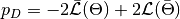 for the method of Spiegelhalter and as
 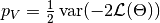 for the method of Gelman. Results are for all chains combined.
Example
See the Posterior Summaries section of the tutorial.
-
logpdf(mc::ModelChains, nodekey::Symbol)¶ -
logpdf(mc::ModelChains, nodekeys::Vector{Symbol}=keys(mc.model, :stochastic)) Compute the sum of log-densities at each iteration of MCMC output for stochastic nodes.
Arguments
mc: sampler output from a model fit with themcmc()function.nodekey/nodekeys: stochastic model node(s) over which to sum densities (default: all).
Value
AModelChainsobject of resulting summed log-densities at each MCMC iteration of the supplied chain.
-
predict(mc::ModelChains, nodekey::Symbol)¶ -
predict(mc::ModelChains, nodekeys::Vector{Symbol}=keys(mc.model, :output)) Generate MCMC draws from a posterior predictive distribution.
Arguments
mc: sampler output from a model fit with themcmc()function.nodekey/nodekeys: observed Stochastic model node(s) for which to generate draws from the predictive distribution (default: all observed data nodes).
Value
A
ModelChainsobject of draws simulated at each MCMC iteration of the supplied chain. For observed data node , simulation is from the posterior predictive distribution
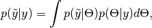
where
 is an unknown observation on the node,
  is the data likelihood, and
  is the posterior distribution of unobserved parameters .
Example
See the Pumps example.
Plotting
-
plot(c::AbstractChains, ptype::Vector{Symbol}=[:trace, :density]; legend::Bool=false, args...)¶ -
plot(c::AbstractChains, ptype::Symbol; legend::Bool=false, args...) Various plots to summarize sampler output stored in
AbstractChainssubtypes. Separate plots are produced for each sampled parameter.Arguments
c: sampler output to plot.ptype: plot type(s). Options are:autocor: autocorrelation plots, with optional argumentmaxlag::Integer=round(Int, 10 * log10(length(c.range)))determining the maximum autocorrelation lag to plot. Lags are plotted relative to the thinning interval of the output.:bar: bar plots. Optional argumentposition::Symbol=:stackcontrols whether bars should be stacked on top of each other (default) or placed side by side (:dodge).:contour: pairwise posterior density contour plots. Optional argumentbins::Integer=100controls the plot resolution.:density: density plots. Optional argumenttrim::Tuple{Real, Real}=(0.025, 0.975)trims off lower and upper quantiles of density.:mean: running mean plots.:mixeddensity: bar plots (:bar) for parameters with integer values within bounds defined by optional argumentbarbounds::Tuple{Real, Real}=(0, Inf), and density plots (:density) otherwise.:trace: trace plots.
legend: whether to include legends in the plots to identify chain-specific results.args...: additional keyword arguments to be passed to theptypeoptions, as described above.
Value
Returns aVector{Plot}whose elements are individual parameter plots of the specified type ifptypeis a symbol, and aMatrix{Plot}with plot types in the rows and parameters in the columns ifptypeis a vector. The result can be displayed or saved to a file withdraw().Note
Plots are created using the Gadfly package [51].Example
See the Plotting section of the tutorial.
-
draw(p::Array{Plot}; fmt::Symbol=:svg, filename::AbstractString="", width::MeasureOrNumber=8inch, height::MeasureOrNumber=8inch, nrow::Integer=3, ncol::Integer=2, byrow::Bool=true, ask::Bool=true)¶ Draw plots produced by
plot()into display grids containing a default of 3 rows and 2 columns of plots.Arguments
p: plots to be drawn. Elements ofpare read in the order stored by julia (e.g. column-major order for matrices) and written to the display grid according to thebyrowargument. Grids will be filled sequentially until all plots have been drawn.fmt: output format. Options are:pdf: Portable Document Format (.pdf).:pgf: Portable Graphics Format (.pgf).:png: Portable Network Graphics (.png).:ps: Postscript (.ps).:svg: Scalable Vector Graphics (.svg).
filename: file to which to save the display grids as they are drawn, or an empty string to draw to the display device (default). If a supplied external file name does not include a dot (.), then a hyphen followed by the grid sequence number and then the format extension will be appended automatically. In the case of multiple grids, the former file name behavior will write all grids to the single named file, but prompt users before advancing to the next grid and overwriting the file; the latter behavior will write each grid to a different file.width/height: grid widths/heights incm,mm,inch,pt, orpxunits.nrow/ncol: number of rows/columns in the display grids.byrow: whether the display grids should be filled by row.ask: whether to prompt users before displaying subsequent grids to a single named file or the display device.
Value
Grids drawn to an external file or the display device.Example
See the Plotting section of the tutorial.