Blocker: Random Effects Meta-Analysis of Clinical Trials
An example from OpenBUGS [44] and Carlin [15] concerning a meta-analysis of 22 clinical trials to prevent mortality after myocardial infarction.
Model
Events are modelled as
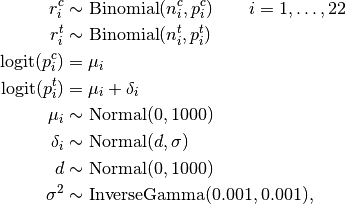
where  is the number of control group events, out of
  , in study
  ; and
; and  is the number of treatment group events.
Analysis Program
using Distributed
@everywhere using Mamba

## Data
blocker = Dict{Symbol, Any}(
  :rt =>
    [3, 7, 5, 102, 28, 4, 98, 60, 25, 138, 64, 45, 9, 57, 25, 33, 28, 8, 6, 32,
     27, 22],
  :nt =>
    [38, 114, 69, 1533, 355, 59, 945, 632, 278, 1916, 873, 263, 291, 858, 154,
     207, 251, 151, 174, 209, 391, 680],
  :rc =>
    [3, 14, 11, 127, 27, 6, 152, 48, 37, 188, 52, 47, 16, 45, 31, 38, 12, 6, 3,
     40, 43, 39],
  :nc =>
    [39, 116, 93, 1520, 365, 52, 939, 471, 282, 1921, 583, 266, 293, 883, 147,
     213, 122, 154, 134, 218, 364, 674]
)
blocker[:N] = length(blocker[:rt])


## Model Specification
model = Model(

  rc = Stochastic(1,
    (mu, nc, N) ->
      begin
        pc = invlogit.(mu)
        UnivariateDistribution[Binomial(nc[i], pc[i]) for i in 1:N]
      end,
    false
  ),

  rt = Stochastic(1,
    (mu, delta, nt, N) ->
      begin
        pt = invlogit.(mu + delta)
        UnivariateDistribution[Binomial(nt[i], pt[i]) for i in 1:N]
      end,
    false
  ),

  mu = Stochastic(1,
    () -> Normal(0, 1000),
    false
  ),

  delta = Stochastic(1,
    (d, s2) -> Normal(d, sqrt(s2)),
    false
  ),

  delta_new = Stochastic(
    (d, s2) -> Normal(d, sqrt(s2))
  ),

  d = Stochastic(
    () -> Normal(0, 1000)
  ),

  s2 = Stochastic(
    () -> InverseGamma(0.001, 0.001)
  )

)


## Initial Values
inits = [
  Dict(:rc => blocker[:rc], :rt => blocker[:rt], :d => 0, :delta_new => 0,
       :s2 => 1, :mu => zeros(blocker[:N]), :delta => zeros(blocker[:N])),
  Dict(:rc => blocker[:rc], :rt => blocker[:rt], :d => 2, :delta_new => 2,
       :s2 => 10, :mu => fill(2, blocker[:N]), :delta => fill(2, blocker[:N]))
]


## Sampling Scheme
scheme = [AMWG(:mu, 0.1),
          AMWG([:delta, :delta_new], 0.1),
          Slice([:d, :s2], 1.0)]
setsamplers!(model, scheme)


## MCMC Simulations
sim = mcmc(model, blocker, inits, 10000, burnin=2500, thin=2, chains=2)
describe(sim)
Results
Iterations = 2502:10000
Thinning interval = 2
Chains = 1,2
Samples per chain = 3750

Empirical Posterior Estimates:
              Mean         SD        Naive SE       MCSE        ESS
       s2  0.01822186 0.021121265 0.00024388736 0.0014150714 222.78358
        d -0.25563567 0.061841945 0.00071408927 0.0040205781 236.58613
delta_new -0.25005767 0.150325282 0.00173580684 0.0050219145 896.03592

Quantiles:
               2.5%         25.0%         50.0%         75.0%       97.5%
       s2  0.0006855452  0.0041648765  0.0107615659  0.024442084  0.07735715
        d -0.3734122953 -0.2959169814 -0.2581848849 -0.218341380 -0.12842580
delta_new -0.5385405488 -0.3279958446 -0.2557849252 -0.177588413  0.07986060