Pumps: Gamma-Poisson Hierarchical Model
An example from OpenBUGS [44] and George et al. [36] concerning the number of failures of 10 power plant pumps.
Model
Pump failure are modelled as
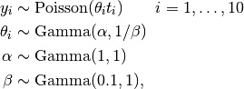
where  is the number of times that pump
  failed, and
  is the operation time of the pump (in 1000s of hours).
Analysis Program
using Distributed
@everywhere using Mamba

## Data
pumps = Dict{Symbol, Any}(
  :y => [5, 1, 5, 14, 3, 19, 1, 1, 4, 22],
  :t => [94.3, 15.7, 62.9, 126, 5.24, 31.4, 1.05, 1.05, 2.1, 10.5]
)
pumps[:N] = length(pumps[:y])


## Model Specification
model = Model(

  y = Stochastic(1,
    (theta, t, N) ->
      UnivariateDistribution[(
        lambda = theta[i] * t[i];
        Poisson(lambda)) for i in 1:N
      ],
    false
  ),

  theta = Stochastic(1,
    (alpha, beta) -> Gamma(alpha, 1 / beta),
    true
  ),

  alpha = Stochastic(
    () -> Exponential(1.0)
  ),

  beta = Stochastic(
    () -> Gamma(0.1, 1.0)
  )

)


## Initial Values
inits = [
  Dict(:y => pumps[:y], :alpha => 1.0, :beta => 1.0,
       :theta => rand(Gamma(1.0, 1.0), pumps[:N])),
  Dict(:y => pumps[:y], :alpha => 10.0, :beta => 10.0,
       :theta => rand(Gamma(10.0, 10.0), pumps[:N]))
]


## Sampling Scheme
scheme = [Slice([:alpha, :beta], 1.0, Univariate),
          Slice(:theta, 1.0, Univariate)]
setsamplers!(model, scheme)


## MCMC Simulations
sim = mcmc(model, pumps, inits, 10000, burnin=2500, thin=2, chains=2)
describe(sim)


## Posterior Predictive Distribution
ppd = predict(sim, :y)
describe(ppd)
Results
## MCMC Simulations

Iterations = 2502:10000
Thinning interval = 2
Chains = 1,2
Samples per chain = 3750

Empirical Posterior Estimates:
             Mean         SD        Naive SE        MCSE         ESS
     beta 0.93036099 0.517274134 0.00597296721 0.01824153419  804.11618
    alpha 0.69679849 0.264420102 0.00305326034 0.00722593007 1339.06428
 theta[1] 0.05991674 0.025050913 0.00028926303 0.00032725274 3750.00000
 theta[2] 0.10125873 0.078887354 0.00091091270 0.00129985769 3683.18182
 theta[3] 0.08910382 0.037307731 0.00043079257 0.00045660986 3750.00000
 theta[4] 0.11529009 0.030274265 0.00034957710 0.00032583333 3750.00000
 theta[5] 0.59971611 0.316811730 0.00365822675 0.00585119652 2931.65686
 theta[6] 0.60967188 0.134761371 0.00155609028 0.00174949908 3750.00000
 theta[7] 0.86767451 0.669943846 0.00773584520 0.02858200254  549.40360
 theta[8] 0.85445727 0.668132036 0.00771492422 0.02485547216  722.57105
 theta[9] 1.55721556 0.753564449 0.00870141275 0.03109274798  587.38464
theta[10] 1.98475207 0.405438843 0.00468160451 0.00912748779 1973.09587

Quantiles:
              2.5%       25.0%      50.0%      75.0%      97.5%
     beta 0.189558591 0.55034346 0.84013720 1.22683690 2.134324768
    alpha 0.286434561 0.50214938 0.66295652 0.85427430 1.319308645
 theta[1] 0.021291808 0.04164372 0.05696335 0.07435302 0.118041776
 theta[2] 0.008789962 0.04279772 0.08116810 0.13771833 0.305675244
 theta[3] 0.032503106 0.06202730 0.08293498 0.11024076 0.176883533
 theta[4] 0.063587574 0.09389172 0.11222268 0.13443866 0.182555751
 theta[5] 0.153474125 0.36947945 0.54009121 0.77234190 1.364481338
 theta[6] 0.371096082 0.51395467 0.60089332 0.69531957 0.898866079
 theta[7] 0.077416146 0.37391993 0.71230582 1.17659703 2.616100803
 theta[8] 0.072479432 0.35973235 0.69319639 1.16347299 2.655857786
 theta[9] 0.463821785 1.01169918 1.43745818 1.96871605 3.351798915
theta[10] 1.269842527 1.70167020 1.95748757 2.24000075 2.861197982

## Posterior Predictive Distribution

Iterations = 2502:10000
Thinning interval = 2
Chains = 1,2
Samples per chain = 3750

Empirical Posterior Estimates:
         Mean        SD      Naive SE      MCSE       ESS
 y[1]  5.5784000 3.3457654 0.038633571 0.042295418 3750.0000
 y[2]  1.6009333 1.7532320 0.020244579 0.022399464 3750.0000
 y[3]  5.5854667 3.2976980 0.038078537 0.040503717 3750.0000
 y[4] 14.5666667 5.4547523 0.062986054 0.061718435 3750.0000
 y[5]  3.1118667 2.4165260 0.027903638 0.035965796 3750.0000
 y[6] 19.0780000 6.0320229 0.069651801 0.071700830 3750.0000
 y[7]  0.9008000 1.1756177 0.013574864 0.031805581 1366.2355
 y[8]  0.8922667 1.1550634 0.013337523 0.025610086 2034.1808
 y[9]  3.2585333 2.4039269 0.027758156 0.069046712 1212.1504
y[10] 20.7933333 6.2068800 0.071670876 0.113975236 2965.6896

Quantiles:
      2.5% 25.0% 50.0% 75.0% 97.5%
 y[1]    1     3     5     8    13
 y[2]    0     0     1     2     6
 y[3]    1     3     5     7    13
 y[4]    5    11    14    18    27
 y[5]    0     1     3     4     9
 y[6]    9    15    19    23    32
 y[7]    0     0     1     1     4
 y[8]    0     0     1     1     4
 y[9]    0     1     3     5     9
y[10]   10    16    20    25    34