Salm: Extra-Poisson Variation in a Dose-Response Study
An example from OpenBUGS [44] and Breslow [9] concerning mutagenicity assay data on salmonella in three plates exposed to six doses of quinoline.
Model
Number of revertant colonies of salmonella are modelled as
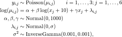
where  is the number of colonies in plate
  and dose
  .
.
Analysis Program
using Distributed
@everywhere using Mamba

## Data
salm = Dict{Symbol, Any}(
  :y => reshape(
    [15, 21, 29, 16, 18, 21, 16, 26, 33, 27, 41, 60, 33, 38, 41, 20, 27, 42],
    3, 6),
  :x => [0, 10, 33, 100, 333, 1000],
  :plate => 3,
  :dose => 6
)


## Model Specification
model = Model(

  y = Stochastic(2,
    (alpha, beta, gamma, x, lambda) ->
      UnivariateDistribution[(
        mu = exp(alpha + beta * log(x[j] + 10) + gamma * x[j] + lambda[i, j]);
        Poisson(mu)) for i in 1:3, j in 1:6
      ],
    false
  ),

  alpha = Stochastic(
    () -> Normal(0, 1000)
  ),

  beta = Stochastic(
    () -> Normal(0, 1000)
  ),

  gamma = Stochastic(
    () -> Normal(0, 1000)
  ),

  lambda = Stochastic(2,
    s2 -> Normal(0, sqrt(s2)),
    false
  ),

  s2 = Stochastic(
    () -> InverseGamma(0.001, 0.001)
  )

)


## Initial Values
inits = [
  Dict(:y => salm[:y], :alpha => 0, :beta => 0, :gamma => 0, :s2 => 10,
       :lambda => zeros(3, 6)),
  Dict(:y => salm[:y], :alpha => 1, :beta => 1, :gamma => 0.01, :s2 => 1,
       :lambda => zeros(3, 6))
]

## Sampling Scheme
scheme = [Slice([:alpha, :beta, :gamma], [1.0, 1.0, 0.1]),
          AMWG([:lambda, :s2], 0.1)]
setsamplers!(model, scheme)


## MCMC Simulations
sim = mcmc(model, salm, inits, 10000, burnin=2500, thin=2, chains=2)
describe(sim)
Results
Iterations = 2502:10000
Thinning interval = 2
Chains = 1,2
Samples per chain = 3750

Empirical Posterior Estimates:
           Mean           SD         Naive SE         MCSE          ESS
   s2  0.0690769709 0.04304237136 0.000497010494 0.001985478741 469.961085
gamma -0.0011250515 0.00034536546 0.000003987937 0.000025419899 184.590851
 beta  0.3543443166 0.07160779229 0.000826855563 0.007122805926 101.069088
alpha  2.0100584321 0.26156942610 0.003020343571 0.027100522461  93.157673

Quantiles:
           2.5%         25.0%        50.0%          75.0%          97.5%
   s2  0.0135820292  0.039788136  0.0598307554  0.08740879470  0.17747300708
gamma -0.0017930379 -0.001347435 -0.0011325733 -0.00090960998 -0.00039271486
 beta  0.2073237562  0.312747679  0.3582979574  0.40006921583  0.48789037325
alpha  1.5060295212  1.847111545  2.0062727893  2.16556036713  2.50547846044