Stacks: Robust Regression

An example from OpenBUGS [44], Brownlee [14], and Birkes and Dodge [5] concerning 21 daily responses of stack loss, the amount of ammonia escaping, as a function of air flow, temperature, and acid concentration.

Model

Losses are modelled as

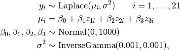
where is the stack loss on day ; and are standardized predictors.

Analysis Program

using Distributed
@everywhere using Mamba

## Data
stacks = Dict{Symbol, Any}(
  :y => [42, 37, 37, 28, 18, 18, 19, 20, 15, 14, 14, 13, 11, 12, 8, 7, 8, 8, 9,
         15, 15],
  :x =>
    [80 27 89
     80 27 88
     75 25 90
     62 24 87
     62 22 87
     62 23 87
     62 24 93
     62 24 93
     58 23 87
     58 18 80
     58 18 89
     58 17 88
     58 18 82
     58 19 93
     50 18 89
     50 18 86
     50 19 72
     50 19 79
     50 20 80
     56 20 82
     70 20 91]
)
stacks[:N] = size(stacks[:x], 1)
stacks[:p] = size(stacks[:x], 2)

stacks[:meanx] = map(j -> mean(stacks[:x][:, j]), 1:stacks[:p])
stacks[:sdx] = map(j -> std(stacks[:x][:, j]), 1:stacks[:p])
stacks[:z] = Float64[
  (stacks[:x][i, j] - stacks[:meanx][j]) / stacks[:sdx][j]
  for i in 1:stacks[:N], j in 1:stacks[:p]
]


## Model Specification
model = Model(

  y = Stochastic(1,
    (mu, s2, N) ->
      UnivariateDistribution[Laplace(mu[i], s2) for i in 1:N],
    false
  ),

  beta0 = Stochastic(
    () -> Normal(0, 1000),
    false
  ),

  beta = Stochastic(1,
    () -> Normal(0, 1000),
    false
  ),

  mu = Logical(1,
    (beta0, z, beta) -> beta0 .+ z * beta,
    false
  ),

  s2 = Stochastic(
    () -> InverseGamma(0.001, 0.001),
    false
  ),

  sigma = Logical(
    s2 -> sqrt(2.0) * s2
  ),

  b0 = Logical(
    (beta0, b, meanx) -> beta0 - dot(b, meanx)
  ),

  b = Logical(1,
    (beta, sdx) -> beta ./ sdx
  ),

  outlier = Logical(1,
    (y, mu, sigma, N) ->
      Float64[abs((y[i] - mu[i]) / sigma) > 2.5 for i in 1:N],
    [1, 3, 4, 21]
  )

)


## Initial Values
inits = [
  Dict(:y => stacks[:y], :beta0 => 10, :beta => [0, 0, 0], :s2 => 10),
  Dict(:y => stacks[:y], :beta0 => 1, :beta => [1, 1, 1], :s2 => 1)
]


## Sampling Scheme
scheme = [NUTS([:beta0, :beta]),
          Slice(:s2, 1.0)]
setsamplers!(model, scheme)


## MCMC Simulations
sim = mcmc(model, stacks, inits, 10000, burnin=2500, thin=2, chains=2)
describe(sim)

Results

Iterations = 2502:10000
Thinning interval = 2
Chains = 1,2
Samples per chain = 3750

Empirical Posterior Estimates:
                 Mean         SD       Naive SE       MCSE        ESS
       b[1]   0.836863707 0.13085145 0.0015109423 0.0027601754 2247.4171
       b[2]   0.744454449 0.33480007 0.0038659382 0.0065756939 2592.3158
       b[3]  -0.116648437 0.12214077 0.0014103601 0.0015143922 3750.0000
         b0 -38.776564595 8.81860433 0.1018284717 0.0979006137 3750.0000
      sigma   3.487643717 0.87610847 0.0101164292 0.0279025494  985.8889
 outlier[1]   0.042666667 0.20211796 0.0023338572 0.0029490162 3750.0000
 outlier[3]   0.054800000 0.22760463 0.0026281519 0.0034398827 3750.0000
 outlier[4]   0.298000000 0.45740999 0.0052817156 0.0089200654 2629.5123
outlier[21]   0.606400000 0.48858046 0.0056416412 0.0113877443 1840.7583

Quantiles:
                2.5%         25.0%        50.0%         75.0%         97.5%
       b[1]   0.57218621   0.75741345   0.834874964   0.918345319   1.101502854
       b[2]   0.16177144   0.52291878   0.714951465   0.933171533   1.476258382
       b[3]  -0.36401372  -0.19028697  -0.113463801  -0.036994963   0.118538277
         b0 -56.70056875 -44.11785905 -38.698338454 -33.409149788 -21.453323631
      sigma   2.17947513   2.86899865   3.348631697   3.953033535   5.592773118
 outlier[1]   0.00000000   0.00000000   0.000000000   0.000000000   1.000000000
 outlier[3]   0.00000000   0.00000000   0.000000000   0.000000000   1.000000000
 outlier[4]   0.00000000   0.00000000   0.000000000   1.000000000   1.000000000
outlier[21]   0.00000000   0.00000000   1.000000000   1.000000000   1.000000000