Epilepsy: Repeated Measures on Poisson Counts¶

An example from OpenBUGS [38], Thall and Vail [71] Breslow and Clayton [9] concerning the effects of treatment, baseline seizure counts, and age on follow-up seizure counts at four visits in 59 patients.

Model¶

Counts are modelled as

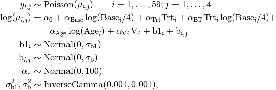
$y_{i,j} &\sim \text{Poisson}(\mu_{i,j}) \quad\quad i=1,\ldots,59; j=1,\ldots,4 \\ \log(\mu_{i,j}) &= \alpha_0 + \alpha_\text{Base} \log(\text{Base}_i / 4) + \alpha_\text{Trt} \text{Trt}_i + \alpha_\text{BT} \text{Trt}_i \log(\text{Base}_i / 4) + \\ & \quad\quad \alpha_\text{Age} \log(\text{Age}_i) + \alpha_\text{V4} \text{V}_4 + \text{b1}_i + \text{b}_{i,j} \\ \text{b1}_i &\sim \text{Normal}(0, \sigma_\text{b1}) \\ \text{b}_{i,j} &\sim \text{Normal}(0, \sigma_\text{b}) \\ \alpha_* &\sim \text{Normal}(0, 100) \\ \sigma^2_\text{b1}, \sigma^2_\text{b} &\sim \text{InverseGamma}(0.001, 0.001),$

where $y_{ij}$ are the counts on patient $i$ at visit $j$ , $\text{Trt}$ is a treatment indicator, $\text{Base}$ is baseline seizure counts, $\text{Age}$ is age in years, and $\text{V}_4$ is an indicator for the fourth visit.

Analysis Program¶

using Mamba

## Data
epil = (Symbol => Any)[
  :y =>
    [ 5  3  3  3
      3  5  3  3
      2  4  0  5
      4  4  1  4
      7 18  9 21
      5  2  8  7
      6  4  0  2
     40 20 21 12
      5  6  6  5
     14 13  6  0
     26 12  6 22
     12  6  8  4
      4  4  6  2
      7  9 12 14
     16 24 10  9
     11  0  0  5
      0  0  3  3
     37 29 28 29
      3  5  2  5
      3  0  6  7
      3  4  3  4
      3  4  3  4
      2  3  3  5
      8 12  2  8
     18 24 76 25
      2  1  2  1
      3  1  4  2
     13 15 13 12
     11 14  9  8
      8  7  9  4
      0  4  3  0
      3  6  1  3
      2  6  7  4
      4  3  1  3
     22 17 19 16
      5  4  7  4
      2  4  0  4
      3  7  7  7
      4 18  2  5
      2  1  1  0
      0  2  4  0
      5  4  0  3
     11 14 25 15
     10  5  3  8
     19  7  6  7
      1  1  2  3
      6 10  8  8
      2  1  0  0
    102 65 72 63
      4  3  2  4
      8  6  5  7
      1  3  1  5
     18 11 28 13
      6  3  4  0
      3  5  4  3
      1 23 19  8
      2  3  0  1
      0  0  0  0
      1  4  3  2],
  :Trt =>
    [0, 0, 0, 0, 0, 0, 0, 0, 0, 0, 0, 0, 0, 0, 0, 0, 0, 0, 0, 0, 0, 0, 0, 0, 0,
     0, 0, 0, 1, 1, 1, 1, 1, 1, 1, 1, 1, 1, 1, 1, 1, 1, 1, 1, 1, 1, 1, 1, 1, 1,
     1, 1, 1, 1, 1, 1, 1, 1, 1],
  :Base =>
    [11, 11, 6, 8, 66, 27, 12, 52, 23, 10, 52, 33, 18, 42, 87, 50, 18, 111, 18,
     20, 12, 9, 17, 28, 55, 9, 10, 47, 76, 38, 19, 10, 19, 24, 31, 14, 11, 67,
     41, 7, 22, 13, 46, 36, 38, 7, 36, 11, 151, 22, 41, 32, 56, 24, 16, 22, 25,
     13, 12],
  :Age =>
    [31, 30, 25, 36, 22, 29, 31, 42, 37, 28, 36, 24, 23, 36, 26, 26, 28, 31, 32,
     21, 29, 21, 32, 25, 30, 40, 19, 22, 18, 32, 20, 30, 18, 24, 30, 35, 27, 20,
     22, 28, 23, 40, 33, 21, 35, 25, 26, 25, 22, 32, 25, 35, 21, 41, 32, 26, 21,
     36, 37],
  :V4 => [0, 0, 0, 1]
]
epil[:N] = size(epil[:y], 1)
epil[:T] = size(epil[:y], 2)

epil[:logBase4] = log(epil[:Base] / 4)
epil[:BT] = epil[:logBase4] .* epil[:Trt]
epil[:logAge] = log(epil[:Age])
map(key -> epil[symbol(string(key, "bar"))] = mean(epil[key]),
    [:logBase4, :Trt, :BT, :logAge, :V4])


## Model Specification

model = Model(

  y = Stochastic(2,
    @modelexpr(a0, alpha_Base, logBase4, logBase4bar, alpha_Trt, Trt, Trtbar,
               alpha_BT, BT, BTbar, alpha_Age, logAge, logAgebar, alpha_V4, V4,
               V4bar, b1, b, N, T,
      Distribution[
        begin
          mu = exp(a0 + alpha_Base * (logBase4[i] - logBase4bar) +
                   alpha_Trt * (Trt[i] - Trtbar) + alpha_BT * (BT[i] - BTbar) +
                   alpha_Age * (logAge[i] - logAgebar) +
                   alpha_V4 * (V4[j] - V4bar) + b1[i] +
                   b[i,j])
          Poisson(mu)
        end
        for i in 1:N, j in 1:T
      ]
    ),
    false
  ),

  b1 = Stochastic(1,
    @modelexpr(s2_b1,
      Normal(0, sqrt(s2_b1))
    ),
    false
  ),

  b = Stochastic(2,
    @modelexpr(s2_b,
      Normal(0, sqrt(s2_b))
    ),
    false
  ),

  a0 = Stochastic(
    :(Normal(0, 100)),
    false
  ),

  alpha_Base = Stochastic(
    :(Normal(0, 100))
  ),

  alpha_Trt = Stochastic(
    :(Normal(0, 100))
  ),

  alpha_BT = Stochastic(
    :(Normal(0, 100))
  ),

  alpha_Age = Stochastic(
    :(Normal(0, 100))
  ),

  alpha_V4 = Stochastic(
    :(Normal(0, 100))
  ),

  alpha0 = Logical(
    @modelexpr(a0, alpha_Base, logBase4bar, alpha_Trt, Trtbar, alpha_BT, BTbar,
               alpha_Age, logAgebar, alpha_V4, V4bar,
      a0 - alpha_Base * logBase4bar - alpha_Trt * Trtbar - alpha_BT * BTbar -
        alpha_Age * logAgebar - alpha_V4 * V4bar
    )
  ),

  s2_b1 = Stochastic(
    :(InverseGamma(0.001, 0.001))
  ),

  s2_b = Stochastic(
    :(InverseGamma(0.001, 0.001))
  )

)


## Initial Values
inits = [
  [:y => epil[:y], :a0 => 0, :alpha_Base => 0, :alpha_Trt => 0,
   :alpha_BT => 0, :alpha_Age => 0, :alpha_V4 => 0, :s2_b1 => 1,
   :s2_b => 1, :b1 => zeros(epil[:N]), :b => zeros(epil[:N], epil[:T])],
  [:y => epil[:y], :a0 => 1, :alpha_Base => 1, :alpha_Trt => 1,
   :alpha_BT => 1, :alpha_Age => 1, :alpha_V4 => 1, :s2_b1 => 10,
   :s2_b => 10, :b1 => zeros(epil[:N]), :b => zeros(epil[:N], epil[:T])]
]


## Sampling Scheme
scheme = [AMWG([:a0, :alpha_Base, :alpha_Trt, :alpha_BT, :alpha_Age,
                :alpha_V4], fill(0.1, 6)),
          Slice([:b1], fill(0.5, epil[:N])),
          Slice([:b], fill(0.5, epil[:N] * epil[:T])),
          Slice([:s2_b1, :s2_b], ones(2))]
setsamplers!(model, scheme)


## MCMC Simulations
sim = mcmc(model, epil, inits, 15000, burnin=2500, thin=2, chains=2)
describe(sim)

Results¶

Iterations = 2502:15000
Thinning interval = 2
Chains = 1,2
Samples per chain = 6250

Empirical Posterior Estimates:
              Mean        SD      Naive SE       MCSE       ESS
 alpha_Age  0.4583090 0.3945362 0.0035288392 0.020336364 376.38053
    alpha0 -1.3561708 1.3132402 0.0117459774 0.072100024 331.75503
  alpha_BT  0.2421700 0.1905664 0.0017044781 0.010759318 313.70641
alpha_Base  0.9110497 0.1353545 0.0012106472 0.007208435 352.58447
      s2_b  0.1352375 0.0318193 0.0002846002 0.001551352 420.68781
 alpha_Trt -0.7593139 0.3977342 0.0035574432 0.023478808 286.96826
     s2_b1  0.2491188 0.0731667 0.0006544231 0.002900632 636.27088
  alpha_V4 -0.0928793 0.0836669 0.0007483393 0.003604194 538.87837

Quantiles:
              2.5%      25.0%      50.0%      75.0%      97.5%
 alpha_Age -0.1966699  0.176356  0.4160869  0.6966479  1.3050754
    alpha0 -4.1688878 -2.157933 -1.2634314 -0.4362265  0.8661958
  alpha_BT -0.0902501  0.108103  0.2265617  0.3583543  0.6578050
alpha_Base  0.6631882  0.817701  0.9026821  0.9974174  1.2006197
      s2_b  0.0715581  0.112591  0.1362650  0.1580326  0.1937159
 alpha_Trt -1.6368221 -1.011391 -0.7565400 -0.4808709 -0.0161134
     s2_b1  0.1381748  0.197135  0.2376114  0.2896550  0.4228051
  alpha_V4 -0.2550453 -0.148157 -0.0931360 -0.0366814  0.0720990