Salm: Extra-Poisson Variation in a Dose-Response Study¶

An example from OpenBUGS [38] and Breslow [8] concerning mutagenicity assay data on salmonella in three plates exposed to six doses of quinoline.

Model¶

Number of revertant colonies of salmonella are modelled as

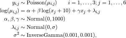
$y_{i,j} &\sim \text{Poisson}(\mu_{i,j}) \quad\quad i=1,\ldots,3; j=1,\ldots,6 \\ \log(\mu_{i,j}) &= \alpha + \beta \log(x_j + 10) + \gamma x_j + \lambda_{i,j} \\ \alpha, \beta, \gamma &\sim \text{Normal}(0, 1000) \\ \lambda_{i,j} &\sim \text{Normal}(0, \sigma) \\ \sigma^2 &\sim \text{InverseGamma}(0.001, 0.001),$

where $y_i$ is the number of colonies in plate $i$ and dose $j$ .

Analysis Program¶

using Mamba

## Data
salm = (Symbol => Any)[
  :y => reshape(
    [15, 21, 29, 16, 18, 21, 16, 26, 33, 27, 41, 60, 33, 38, 41, 20, 27, 42],
    3, 6),
  :x => [0, 10, 33, 100, 333, 1000],
  :plate => 3,
  :dose => 6
]


## Model Specification

model = Model(

  y = Stochastic(2,
    @modelexpr(alpha, beta, gamma, x, lambda,
      Distribution[
        begin
          mu = exp(alpha + beta * log(x[j] + 10) + gamma * x[j] + lambda[i,j])
          Poisson(mu)
        end
        for i in 1:3, j in 1:6
      ]
    ),
    false
  ),

  alpha = Stochastic(
    :(Normal(0, 1000))
  ),

  beta = Stochastic(
    :(Normal(0, 1000))
  ),

  gamma = Stochastic(
    :(Normal(0, 1000))
  ),

  lambda = Stochastic(2,
    @modelexpr(s2,
      Normal(0, sqrt(s2))
    ),
    false
  ),

  s2 = Stochastic(
    :(InverseGamma(0.001, 0.001))
  )

)


## Initial Values
inits = [
  [:y => salm[:y], :alpha => 0, :beta => 0, :gamma => 0, :s2 => 10,
   :lambda => zeros(3, 6)],
  [:y => salm[:y], :alpha => 1, :beta => 1, :gamma => 0.01, :s2 => 1,
   :lambda => zeros(3, 6)]
]

## Sampling Scheme
scheme = [Slice([:alpha, :beta, :gamma], [1.0, 1.0, 0.1]),
          AMWG([:lambda, :s2], fill(0.1, 19))]
setsamplers!(model, scheme)


## MCMC Simulations
sim = mcmc(model, salm, inits, 10000, burnin=2500, thin=2, chains=2)
describe(sim)

Results¶

Iterations = 2502:10000
Thinning interval = 2
Chains = 1,2
Samples per chain = 3750

Empirical Posterior Estimates:
         Mean        SD       Naive SE     MCSE       ESS
gamma -0.0011251 0.00034537 0.000003988 0.00002158 256.1352
alpha  2.0100584 0.26156943 0.003020344 0.02106994 154.1158
   s2  0.0690770 0.04304237 0.000497010 0.00192980 497.4697
 beta  0.3543443 0.07160779 0.000826856 0.00564423 160.9577

Quantiles:
         2.5%       25.0%     50.0%      75.0%      97.5%
gamma -0.0017930 -0.0013474 -0.001133 -0.0009096 -0.0003927
alpha  1.5060295  1.8471115  2.006273  2.1655604  2.5054785
   s2  0.0135820  0.0397881  0.059831  0.0874088  0.1774730
 beta  0.2073238  0.3127477  0.358298  0.4000692  0.4878904